Trees
So far we have learned about arrays, stacks, queues and linked lists, which are known as linear data structures. These are termed as linear because the elements are arranged in a linear fashion (that is, one-dimensional representation). Another very useful data structure is tree, where elements appear in a non-linear fashion, which require two-dimensional representation. Figure 8.1 is an example of such a representation.

Fig. 8.1 Tree — a
non-linear representation of data.
There
are numerous examples where tree structure is the efficient means to maintain
and manipulate data. In general, where the hierarchy relationship among data
are to be preserved, tree is used. Figure 8.2 shows a family hierarchy of
various members as a tree which maintains the relationship among them.
This
hierarchy not only gives the ancestors and successors of a family member, but
some other information too. For example, if we assume left side member as
female and right side member as male then sister, brother, uncle, aunt,
grandfather, grandmother, etc. can also be implied automatically.
As an
another example, let us consider an algebraic expression
X
= (A – B)/((C * D) + E)
where, different operators have their own precedence
value. A tree structure to represent the same is shown in Figure 8.3. Here,
operations having the highest precedence are in the lowest level; which
operands are for which operator everything are stated explicitly. Moreover,
associativity can easily be imposed if we place the operators at the left or
right side.
These
two examples illustrate how powerful this data structure is to maintain a lot
of information automatically. Not only these, there are another advantages of
this data structure; insertion, deletion, searching, etc., are more efficient
in trees than the linear data structures.
Before
going to study this data structure, let us introduce the basic terminologies of
tree which will be referred to in subsequent discussions.

Fig. 8.2 A family hierarchy in the form of a
tree.

Fig. 8.3 An algebraic expression in the form
of a tree.
Basic
terminologies
Node. This
is the main component of any tree structure. The concept of node is same as
used in linked list. Node of a tree stores the actual data and links to
the other node. Figure 8.4(a) represents the structure of a node.
Parent. Parent
of a node is the immediate predecessor of a node. Here, X is the parent
of Y and Z. See Figure 8.4(b).
Child. If the immediate predecessor of a node is the parent of the node
then all immediate successors of a node are known as child. For example,
in Figure 8.4(b), Y and Z are the two child of X. Child
which is at the left side called the left child and that of at the right
side is called the right child.
Link. This is a pointer to a node
in a tree. For example, as shown in Figure 8.4(a), LC and RC are two links
of a node. Note that there may be more than two links of a node.
Root. This is a specially
designated node which has no parent. In Figure 8.4(c), A is the root
node.
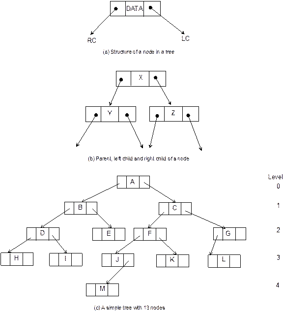
Fig.
8.4 A
tree and its various components.
Leaf. The node which is at the end
and which does not have any child is called leaf node. In Figure 8.4(c),
H, I, K, L, and M are the leaf nodes. Leaf node is also
alternatively termed as terminal node.
Level. Level is the rank of the hierarchy and root node is termed as
in level 0. If a node is at level l then its child is at level l + 1 and parent is at level l
– 1. This is true for all nodes except the root node. Level of the root node is
zero. In Figure 8.4(c), levels of various nodes are depicted.
Height. Maximum number of nodes that
is possible in a path starting from root node to a leaf node is called the height
of a tree. For example, in Figure 8.4(c), the longest path is A – C
– F – J – M and hence the height of this tree is 5. It can
be easily obtained that h = lmax + 1, where h is the height and lmax is the maximum level of the
tree.
Degree. Maximum number of children
that is possible for a node is known as the degree of a node. For
example, the degree of each node of the tree as shown in Figure 8.4(c) is 2.
Sibling. The nodes which have the
same parent are called siblings. For example, in
Figure 8.4(c), J and K are siblings.
Different
text use different term for the above said terms, such as depth for
height, branch or edge for link, arity for degree, external
node for leaf node and internal node for node other than leaf node.
Definition
and Concepts
Let us define a tree. A tree is a finite set
of one or more nodes such that:
(i)
there is a specially designated node called the root,
(ii)
remaining nodes are partitioned into n (n > 0) disjoint sets T1, T2, . . ., Tn, where each Ti (i = 1, 2, . . ., n)
is a tree; T1, T2, . . ., Tn are called subtrees of the
root.
To illustrate the above
definition, let us consider the sample tree as given in Figure 8.6.
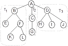
Fig. 8.6 A sample tree T.
In the sample tree T, there is a set of 12 nodes. Here A is a
special node being the root of the tree. Remaining nodes are partitioned into 3
sets T1, T2, and T3; they are sub-trees of the
root node A. By definition, each sub-tree is again a tree. Observe that
a tree is defined recursively. A same tree can be expressed in a string
notation as shown below:
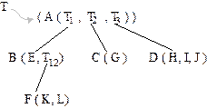
Or more precisely,
T
= (A(B(E, F(K, L))), C(G),
D(H, I, J))
Binary Trees
A binary tree is a special form of a tree.
Contrary to a general tree, a binary tree is more important and frequently used
in various application of computer science. Likewise a general tree, a binary
tree can also be defined as:
A binary tree T is a
finite set of nodes, such that
(i) T
is empty (called empty binary tree), or
(ii) T contains a specially designated node
called the root of T, and the remaining nodes of T form two
disjoint binary trees T1 and T2 which are called left sub-tree and the right
sub-tree respectively.
Figure 8.7
depicts a sample binary tree.
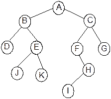
Fig. 8.7 A sample binary tree with 11 nodes.
One can
easily notice the main difference between the definitions of tree and binary
tree. A tree can never be empty but binary tree may be empty. Another
difference is that in case of a binary tree a node may have at most two
children (that is, a tree having degree = 2), whereas in case of a tree, a node
may have any number of children.
Two
special situations of a binary tree are possible: full binary tree and complete
binary tree.
Full binary tree
A binary tree is a full binary tree, if it
contains maximum possible number of nodes in all level. Figure 7.8(a) shows
such a tree with height 4.
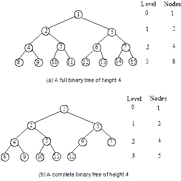
Fig. 8.8 Two special cases of binary trees.
Complete binary tree
A binary tree is said to be a complete binary
tree, if all its level, except possibly the last level, have the maximum number
of possible nodes, and all the nodes at the last level appear as far left as
possible. Figure 7.8(b) depicts a complete binary tree.
Observe
that binary tree as represented in Figure 8.7 is neither a full binary tree nor
a complete binary tree.
Properties of Binary Tree
Binary tree possesses a number of properties. These
properties are very much useful to study further. These properties are listed
below as Lemmas 8.1–8.7.
|
Lemma 8.1 |
|
In any
binary tree, maximum number of nodes on level l is 2l, where l ³ 0. |
Proof: The proof of the above lemma can be done
by induction on l. The root is the only node on level l = 0.
Hence, the maximum number of nodes on level l = 0 is 20 = 1 = 2l.
Suppose,
for all i, 0 £ i < l and for some l, the
above formula is true, that is, the maximum number of nodes at level i
is 2i. Since each node in a
binary tree has degree 2, so from each node at level i, there may be at
most 2 nodes at level i + 1. Thus, the maximum number of nodes at level i
+ 1 is 2 ´ 2i = 2i+1 Therefore, if the formula is true for any i,
then it is also true for i + 1.
Hence,
the proof (see Figure 8.9).
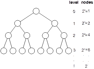
Fig. 8.9 Binary tree showing Lemma 7.1.
|
Lemma 8.2 |
|
Maximum number of nodes possible in a binary tree of height h
is 2h – 1. |
Proof: Maximum number of nodes is possible in a binary
tree, if maximum number of nodes are present in each level. Thus, maximum
number of nodes in a binary tree of height h is
![]() (where lmax is the maximum level of the
tree)
(where lmax is the maximum level of the
tree)
![]() (using the formula of a geometric
series)
(using the formula of a geometric
series)
![]()
From the definition of height, we have h = lmax + 1, hence we can write
nmax = 2h – 1
(7.1)
|
Lemma 8.3 |
|
Minimum number of nodes possible in a binary tree of height h
is h. |
Proof: A binary tree has minimum number of
nodes if each level has minimum number of nodes. Minimum nodes possible at
every level is only one when every parent has one child. Such kind of trees
called skew binary trees are shown in Figure 8.10.

Fig. 8.10 Skew binary trees containing
minimum number of nodes.
Thus, a
skew binary tree is the tree having only one path which contains h
number of nodes if h is its height. Hence nmin = h.
|
Lemma 8.4 |
|
For any
non-empty binary tree, if n is the number of nodes and e is the
number of edges, then n = e + 1. |
Proof: By induction method, we have
Number of nodes, n Number of edge
e n = e +
1
1 0 1 = 0 + 1
2 1 2 = 1 + 1
3 2 3 = 2 + 1
4 3 4 = 3 + 1
. . .
. . .
. . .
n¢ n¢
– 1 n¢ = (n¢
– 1) + 1
Continuing
this, let the above is true for any number of nodes n¢. Thus, n¢ = e¢ + 1.
Now, if
we add one more node into the binary tree having n¢ nodes, then it will
increase one more edge in the binary tree. Thus,
n¢ + 1 = (e¢ + 1) + 1
or
n¢ + 1 = ((n¢ – 1) + 1) + 1
where e¢ = n¢ – 1, therefore
n¢ + 1 = (n¢ + 1 – 1) + 1
This implies that, if the formula is true for any n,
then it is also true for n + 1. Hence, n =
e + 1 is true.
|
Lemma 8.5 |
|
For any non-empty binary tree T,
if n0 is the number of leaf
nodes (degree = 0) and n2 is the number of internal node (degree = 2), then
n0 = n2 + 1. |
Proof Suppose, n be the total number of
nodes in T and ni be the number of nodes having degree i, 0 £ i £ 2. So, we have
n
= n0 + n1 + n2
as T is a binary tree and no other kind of
nodes are possible.
If e
be the number of edge in T then,
e
= n0
´
0 + n1 ´ 1 + n2 ´ 2
or
e
= n1 + 2n2
Again, from Lemma 7.4, we have
n
= e + 1
Thus, from (ii) and (iii), we can write
n
= 1 + n1 + 2n2
And from (i) and (iv), we have
n0 + n1 + n2 = 1 + n1 + 2n2
or
n0 = n2 + 1
Hence the result.
|
Lemma 8.6 |
|
Height
of a complete binary tree with n number of nodes is élog2(n + 1)ù. |
Proof Let h be the height of the
complete binary tree. Then we can write the following inequality:
n
£
20 + 21 + 22 + . . . + 2h–1
or
n £ 2h – 1
or
2h ³ n + 1
Taking logarithm on both sides, we get
h
³
log2(n + 1)
or
h = élog2(n + 1)ù
Hence, the result.
|
Lemma 8.7 |
|
Total
number of binary tree possible with n nodes is |
Proof Proof of this lemma is beyond the scope
of this book;
Representation of Binary Tree
A (binary) tree must represent a hierarchical
relationship between a parent node and (at most two) child nodes. There are two
common methods used for representing this conceptual structure. One is
implicitly: where we do not require the overhead of maintaining pointers
(links) is called linear (or sequential) representation,
using an array. The other is explicitly: known as linked representation,
using pointers. Whatsoever be the representation, the main objective is that
one should have direct access to the root node of the tree, and for given any
node, one should have direct access to the children of it.
Linear Representation of a Binary
Tree
This type of representation is static in the sense
that a block of memory for an array is to be allocated before going to store
the actual tree in it, and once the memory is allocated, the size of the tree
will be restricted as the memory permits.
In this
representation, the nodes are stored level by level, starting from the zero
level where only root node is present. Root node is stored in the first memory
location (as the first element in the array).
Following
rules can be used to decide the location of any node of a tree in the array
(assuming that array index starts from 1):
1. The root node is at location 1.
2. For any node with index i, 1 < i £ n, (for some n):
(a) PARENT(i) = ![]()
For
the node when i = 1, there is no parent.
(b) LCHILD(i) = 2 * i
If
2 *
i > n,
then i has no left child.
(c) RCHILD(i) = 2 * i + 1
If 2 * i + 1 > n,
then i has no right child.
For an example, let us consider the case of
representation of the following expression in the form of a tree:
(A
– B) + C * (D/E)
The binary tree will appear as in Figure 8.11(a).
The representation of the same tree using array is shown in Figure 8.11(b).

Fig. 8.11 Sequential representation of
a binary tree.
Next question arises is how can be the
size of an array estimated? This value can be obtained easily if the binary
tree is a full binary tree. As we know, from Lemma 2, a binary tree of height h
can have at most 2h – 1 nodes. So, the size of
the array to fit such a binary tree is 2h – 1.
To
understand this, a full binary tree and the index of its various nodes when
stored in an array is illustrated as shown in Figure 8.12.

Fig. 8.12 A full binary tree of height
= 4 and label of the nodes represents array locations of nodes.
One can
easily realize the fact that if the tree is a full binary tree then there will
be an efficient use of storage in the array representation (no array location
will be left empty); on the other hand, for a binary tree other than full
binary tree there is a wastage of memory.
Lemma 8.8
gives us the estimation about the maximum and minimum size of the array to
store a binary tree with n nodes.
|
Lemma 8.8 |
|
Maximum
and minimum size that an array may require to store a binary tree with n number
of nodes are Sizemax = 2n – 1
Sizemin =
2 élog2(n+1)ù – 1
|
Proof : If the height
of a binary tree denotes the maximum number of nodes in the longest path of the
tree, then for a tree with n nodes, the maximum height possible is hmax = n. Such a binary
tree is termed as skew binary tree (see Figure 8.13).

Fig. 8.13 A skew binary tree with
maximum height.
If we
store such a binary tree, then it can be seen that the first location is for
the root node, third location (22 – 1) for right child of root node (second node) 7th
(23 – 1) location for the right
child of the second node (third node), and so on. Thus, for a node at level i—it
is actually (i + 1)-th node—its location in the array is at 2i+1 – 1. So, the last node (n-th
node) which is at (n – 1)-th level will be at 2n – 1. This is therefore the
maximum size of the array. Hence,
Sizemax = 2n – 1
Now,
when the tree is a full (or complete) binary tree, then we need minimum sized
array to accommodate the entire tree. In the case of a full or complete binary
tree, with n nodes, minimum height that is possible, is hmin = élog2(n + 1)ù. In that case, the last
element will be stored at ![]() -th
location. Hence the minimum size required is
-th
location. Hence the minimum size required is
![]()
Note: The maximum and minimum size of an array
required to store a binary tree can be expressed in general as:
Size
= 2h – 1
where h be the height of the binary tree.
Here, if h is minimum then minimum sized array and if h is
maximum then maximum sized array will be computed.
Advantages of sequential representation of binary tree
Advantages of the sequential representation of a
binary tree are:
1. Any
node can be accessed from any other node by calculating the index and this is
efficient from execution point of view.
2. Here,
data are stored only without any pointers to their successor or ancestor which
are mentioned implicitly.
3. Programming
languages, where dynamic memory allocation is not possible (such as BASIC,
FORTRAN), array representation is the only means to store a tree.
Disadvantages of sequential representation of binary tree
With these potential advantages, there are
disadvantages as well. These are:
1. Other
than full binary trees, majority of the array entries may be empty.
2. It
allows only static representation. It is no way possible to enhance the tree
structure if the array size is limited.
3. Inserting
a new node to it or deleting a node from it are inefficient with this
representation, because these require considerable data movement up and down
the array which demand excessive amount of processing time.
Linked
Representation of Binary Tree
In spite of simplicity and ease of implementation,
linear representation of binary trees has a number of overheads. In linked
representation of binary trees, all these overheads are taken care of. Linked
representation assumes the structures of a node as shown in Figure 8.15.

Fig. 8.15 Structure of a node in linked
representation.
Here LC
and RC are two link fields to store the address of left child and right child
of a node; DATA is the information content of the node. With this
representation, if one knows the address of the root node then from it any
other node can be accessed. The two forms, that is, ‘tree’ structure and
‘linked’ structure looks almost similar. This similarity implies that the
linked representation of a binary tree very closely resembles the logical
structure of the data involved. This is why, all the algorithms for various
operations with this representation can be easily defined.
Using
the linked representation, the tree with 9 nodes given in Figure 8.16(a) will
appear as shown in Figure 8.16(b)–(c).
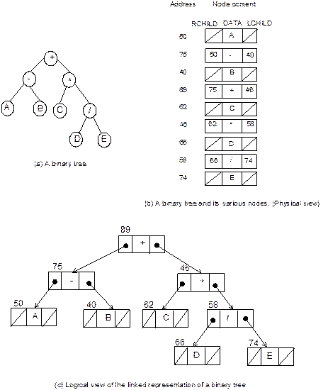
Fig. 8.16 Linked representation of a
binary tree.
Another
advantage of this representation is that it allows dynamic memory allocation;
hence size of the tree can be changed as and when need arises without any limitation
except the limitation of the availability of the total memory.
However,
so far memory requirement for a tree is concerned, it uses more memory than
that the linear representation. Linked representation requires extra memory to
maintain the pointers. Some pointers though with null values, still it needs to
store them. Lemma 8.9 estimates the number of such null links in a binary tree.
|
Lemma 8.9 |
|
In a linked representation of a binary
tree, if there are n number of nodes then the number of null links l = n + 1. |
Proof: By the method of induction. Let R
be the pointer to the root node of a binary tree T. If T is
empty, that is n = 0 then R = null, thus the number of null link l = 0 + 1 = n + 1. For
a single node, that is n = 1, l = 2 = 1 + 1 = n + 1.
Similarly, for a tree T having two nodes, l = 3 = 2 + 1 = n
+ 1. Here it is true for n = 2. Thus, the formula is true for n =
0, 1 and 2 (see Figure 8.17). Let it be true for any n = m.
Therefore, we can write l = m + 1. Now, if we
add one more node into T with m nodes, then number of nodes will
be n¢ = m + 1. Addition of the new node changes
one null link into a non-null value whereas it incorporates two null links of
its own; thus the net increase in null link by this new node is 1. Hence we
have
l = (m
+ 1) + 1 or l = n¢ + 1. This shows that if the
formula is true for m then it is also true for m + 1. As m
is an arbitrary number, the above relation is proved.
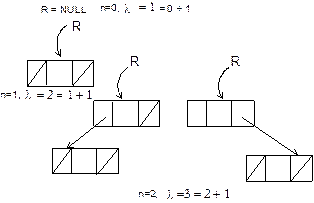
Fig. 8.17 Induction for l = n + 1 when n
= 0, 1 and 2
Physical
Implementation of Binary Tree in Memory
In this section, we will see how simple it is to
implement a binary tree either using sequential (array) or linked
representation. In fact, implementation is just a straightforward translation
from definition of a binary tree to algorithmic description.
The
algorithm BuildTree_1(...) is to
build a tree using an array of element type DATA and the algorithm BuildTree_2 (...) is to build a tree
using linked structure. Both the algorithm will build a tree with user interaction.
Algorithm
BuildTree_1 (...) assumes an array A
of suitable size to store all the data elements in a binary tree. Algorithm BuildTree_2 (...) assumes the node
structure which is same as stated in Section 7.3.2. Both the algorithms follow
recursive definition.
Algorithm BuildTree_1
Input: ITEM is the data content of the node
I. //A binary
tree currently with node at I
Output: A binary tree
with two sub-trees of node I.
Data
structure: Array
representation of tree.
Steps:
|
1. |
If (I ¹ 0) then
// If the tree is
not empty |
||
|
2. |
|
A[I] = ITEM // Store the content of the node
I into the array A |
|
|
3. |
|
Node I has left sub-tree (Give option =
Y/N)? |
|
|
4. |
|
If (option = Y) then // If node I has left sub tree |
|
|
5. |
|
|
BuildTree_1 (2 * I, NEWL) // Then it is at 2*I with next item as NEWL |
|
6. |
|
Else |
|
|
7. |
|
|
BuildTree_1 (0, NULL) // Empty
sub-tree |
|
8. |
|
EndIf |
|
|
9. |
|
Node I has right sub-tree (Give option =
Y/N)? |
|
|
10. |
|
If (option = Y)
// If node I has right sub-tree |
|
|
11. |
|
|
BuildTree_1 (2*I+1, NEWR) //Then it is at 2*I+1 with next item as NEWR |
|
12. |
|
Else |
|
|
13. |
|
|
BuildTree_1 (0, NULL) // Empty
sub-tree |
|
14. |
|
EndIf |
|
|
15. |
EndIf |
||
|
16. |
Stop |
||
Algorithm BuildTree_2
Input: ITEM is the content of the node with
pointer PTR.
Output: A binary tree
with two sub-trees of node PTR.
Data
structure: Linked
list structure of binary tree.
Steps:
|
1. |
If (PTR ¹ NULL) then
// If
the tree is not empty |
||
|
2. |
|
PTR→DATA = ITEM // Store the content of node at
PTR |
|
|
3. |
|
Node PTR has left sub-tree (Give option = Y/N)? |
|
|
4. |
|
If (option = Y) then |
|
|
5. |
|
|
lcptr = GetNode(NODE) // Allocate memory for the left child |
|
6. |
|
|
PTR→LC = lcptr // Assign it to Left link |
|
7. |
|
|
BuildTree_2 (lcptr, NEWL) // Build left sub-tree with next item as
NEWL |
|
8. |
|
Else |
|
|
9. |
|
|
lcptr = NULL |
|
10. |
|
|
PTR→LC = NULL // Assign for an empty left
sub-tree |
|
11. |
|
|
BuildTree_2(lcptr, NULL) //
Empty sub-tree |
|
12. |
|
EndIf |
|
|
13. |
|
Node PTR has right sub-tree (give option = Y/N)? |
|
|
14. |
|
If (option = Y) then |
|
|
15. |
|
|
rcptr = GetNode
(NODE) // Allocate memory for the
right child |
|
16. |
|
|
PTR→RC = rcptr // Assign it
to Right link |
|
17. |
|
|
BuildTree_ 2(rcptr, NEWR)
// Build right sub-tree with next item as NEWR |
|
18. |
|
Else |
|
|
19. |
|
|
rcptr = NULL |
|
20. |
|
|
PTR→RC = NULL // Assign for an empty right
sub-tree |
|
21. |
|
|
BuildTree_ 2(rcptr, NULL) |
|
22. |
|
EndIf |
|
|
23. |
EndIf |
||
|
24. |
Stop |
||
Operations
on Binary Tree
Major operations on a binary tree can be listed as:
1. Insertion. To
include a node into an existing (may be empty) binary tree.
2. Deletion. To
delete a node from a non-empty binary tree.
3. Traversal. To
visit all the nodes in a binary tree.
4. Merge. To
merge two binary trees into a larger one.
Some other special operations are also known for
special cases of binary trees. These will be mentioned later on. Now, let us
discuss the above mentioned operations for general binary trees.
Insertion
With this operation, a new node can be inserted into
any position in a binary tree. Inserting a node as an internal node is
generally based on some criteria which is usually in context of a special form
of a binary tree. We will discuss here a simple case of insertion as external
nodes. Figure 8.18 shows how a node containing data content as G can be
inserted as a left child of a node having data content E. Two algorithms
for two different storage of representations (viz., sequential storage and
linked storage) are stated below.
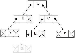
Fig. 8.18 Insertion of a node as an
external node into a binary tree.
Insertion
procedure, in fact, is a two-step process: first to search for the existence of
a node in the given binary tree after which an insertion to be made, and second
is to establish a link for the new node.
Insertion into a sequential representation of a binary tree (as a leaf node)
The following algorithm uses a recursive procedure Search_SEQ to search for a node
containing data as KEY.
Algorithm InsertBinaryTree_SEQ
Input: KEY be the data of a node after which a
new node has to be inserted with data as ITEM.
Output: Newly inserted
node with data as ITEM as a left or
right child of the node with data KEY.
Data
structure: Array
A storing the binary tree.
Steps:
|
1. |
l = Search_SEQ(1, KEY) // Search for the key node in the tree |
||||
|
2. |
If (l = 0) then |
||||
|
3. |
|
Print “Search is unsuccessful :
No insertion” |
|||
|
4. |
|
Exit |
|||
|
5. |
EndIf // Quit the execution |
||||
|
6. |
If (A[2 * l]
= NULL) or (A[2 * l + 1]
= NULL) then
// If the key node has
empty link(s) |
||||
|
7. |
|
Read option to read as left (L) or right (R) // child (give option
= L/R) |
|||
|
8. |
|
If (option = L) then |
|||
|
9. |
|
|
If A[2 * l] = NULL then // Left
link is empty |
||
|
10. |
|
|
|
A[2 * l] = ITEM // Store it in
the array A |
|
|
11. |
|
|
Else // Cannot be inserted as left
child |
||
|
12. |
|
|
|
Print “Desired insertion is not
possible” // as it already has a left child |
|
|
13. |
|
|
|
Exit // Return to the end of the
procedure |
|
|
14. |
|
|
EndIf |
||
|
15. |
|
EndIf |
|||
|
16. |
|
If (option = R) then
//
Move to the right side |
|||
|
17. |
|
|
If (A[2 * l + 1] = NULL) then // Right link is
empty |
||
|
18. |
|
|
|
A[2 * l + 1] = ITEM // Store it in
the array A |
|
|
19. |
|
|
Else
// Cannot be inserted as
right child |
||
|
20. |
|
|
|
Print ‘Desired operation is not
possible’ //as it already has a left child |
|
|
21. |
|
|
|
Exit // Return to the end of the
procedures |
|
|
22. |
|
|
EndIf |
||
|
23. |
|
EndIf // Key node is having both
the child |
|||
|
24. |
Else
// Key node does not have
any empty link |
||||
|
25. |
|
Print “ITEM cannot be inserted
as a leaf node” |
|||
|
26. |
EndIf |
||||
|
27. |
Stop |
||||
The procedure Search_SEQ(. . .) can be defined
recursively as below:
Algorithm Search_SEQ
Input: KEY be the item of search, INDEX being the index of the node from
where searching will start.
Output: LOCATION, where the item KEY is located, if any.
Data
structure: Array
A storing the binary tree. SIZE denotes the size of A.
Steps:
|
1. |
i = INDEX
// Start from root node |
||||
|
2. |
If (A[i] ¹ KEY) then // The present node is not the key node |
||||
|
3. |
|
If (2 * i £ SIZE) then // If left sub-tree is not
exhausted |
|||
|
4. |
|
|
Search_SEQ(2 * i, KEY) //
Search in the left sub-tree |
||
|
5. |
|
Else
// Left sub-tree is exhausted and KEY not found |
|||
|
6. |
|
|
If (2 * i + 1 £ SIZE) then // If right sub-tree is not
exhausted |
||
|
7. |
|
|
|
Search_SEQ (2 * i + 1,
KEY) // Search in the right sub-tree |
|
|
8. |
|
|
Else // The KEY is found neither in left nor
in right sub-tree |
||
|
9. |
|
|
|
Return(0) // Return NULL address for
unsuccessful search |
|
|
10. |
|
|
EndIf |
||
|
11. |
|
EndIf |
|||
|
12. |
Else |
||||
|
13. |
|
Return(i) // Return the address where KEY is found |
|||
|
14. |
EndIf |
||||
|
15. |
Stop |
||||
Insertion into a linked representation of a binary tree (as a leaf node)
Let us assume the node structure used in linked
representation.
Algorithm InsertBinaryTree_LINK
Input: KEY, the data content of the key node
after which a new node is to be inserted and ITEM is the data
content
of the new node that has to be inserted.
Output: A node with data component
ITEM inserted as an external node after the node having data as
KEY if such a node exist with empty link(s), that is, either or both
children is/are absent.
Data
structure: Linked
structure of binary tree. ROOT is the pointer to the root node.
Steps:
|
1. |
ptr
= Search_LINK(ROOT, KEY) |
|||
|
2. |
If (ptr = NULL) then |
|||
|
3. |
|
Print “Search is unsuccessful:
No insertion” |
||
|
4. |
|
Exit |
||
|
5. |
EndIf |
|||
|
6. |
If (ptr→LC = NULL) or (ptr→RC = NULL) //
If either or both link(s) is/are empty |
|||
|
7. |
|
Read
option to insert as left (L) or right (R) child (give option = L/R) |
||
|
8. |
|
If (option = L) then // To
insert as left child |
||
|
9. |
|
|
If (ptr→LC = NULL) then // If the left link is empty then
insert |
|
|
10. |
|
|
|
new
= GetNode(NODE) |
|
11. |
|
|
|
new→DATA = ITEM |
|
12. |
|
|
|
new→LC = new→RC = NULL |
|
13. |
|
|
|
ptr→LC = new |
|
14. |
|
|
Else // The key node already has
left child |
|
|
15. |
|
|
|
Print “Insertion is not
possible as left child” |
|
16. |
|
|
|
Exit // Quit the
execution |
|
17. |
|
|
EndIf |
|
|
18. |
|
Else
//
If option = R) |
||
|
19. |
|
|
If (ptr→RC = NULL) // If the right link is empty then
insert |
|
|
20. |
|
|
|
new
= GetNode (NODE) |
|
21. |
|
|
|
new→DATA = ITEM |
|
22. |
|
|
|
new→LC = new→RC = NULL |
|
23. |
|
|
|
ptr→RC = new |
|
24. |
|
|
Else
// The key node already has right child |
|
|
25. |
|
|
|
Print “Insertion is not
possible as right child” |
|
26. |
|
|
|
Exit // Quit
the execution |
|
27. |
|
|
EndIf |
|
|
28. |
|
Else |
||
|
29. |
|
|
Print “The key node already has
child” //The key node has no empty
child |
|
|
30. |
|
EndIf |
||
|
31. |
EndIf |
|||
|
32. |
Stop |
|||
This algorithm uses a procedure Search_LINK to search for a node containing data as KEY, this procedure can be defined
recursively as below:
Algorithm Search_LINK
Input: KEY, the item of search, PTR0
is the pointer to the linked list from where the search will start.
Output: LOCATION, where the item KEY
is located, if such ITEM exists.
Data structure: Linked structure of
binary tree having ROOT as the pointer to the root node.
Steps:
|
1. |
ptr = PTR0
// Start from a given node |
||
|
2. |
If (ptr→DATA ¹ KEY) // If the current node is not the key node |
||
|
3. |
|
If (ptr→LC ¹ NULL) // If the node has left
sub-tree |
|
|
4. |
|
|
Search_LINK(ptr→LC) // Search the left sub-tree |
|
5. |
|
Else // Key is not in the
left sub-tree |
|
|
6. |
|
|
Return(0) |
|
7. |
|
EndIf |
|
|
8. |
|
If (ptr→RC ¹ NULL) // If the node has right sub-tree |
|
|
9. |
|
|
Search_LINK(ptr→RC) // Search
the right sub-tree |
|
10. |
|
Else // Key is not in the right
sub-tree |
|
|
11. |
|
|
Return(0) // Return
null pointer |
|
12. |
|
EndIf |
|
|
13. |
Else |
||
|
14. |
|
Return(ptr) // Return the pointer to the key node |
|
|
15. |
EndIf |
||
|
16. |
Stop |
||
Deletion
This operation is used to delete any node from any
non-empty binary tree. Likewise the insertion, deletion operation also varies
from one kind of binary trees to another. Deletion operations in various cases
of binary trees will be discussed in due time. Here, we will consider the case
of deletion of leave node in any binary tree. Figure 8.19 shows how a node
containing data as G can be deleted from a binary tree.

Fig. 8.19 Deletion of an external node
in a binary tree.
Let us
see how the deletion operation can be carried out for two kind of storage
representation of binary trees. In order to delete a node in a binary tree, it
is required to reach at the parent node of the node to be deleted. The link
field of the parent node which stores the location of the node to be deleted is
then set by a NULL entry. Let us discuss the algorithm individually.
Deleting a leave node from sequential representation of binary trees
Let SIZE
be the total length of the array A, where binary tree is stored. The
element that has to be deleted is ITEM.
Algorithm DeleteBinTree_SEQ
Input: Given ITEM as data of the node with which the
node can be identified for deletion.
Output: A binary tree
without a node having data as ITEM.
Data
structure: Array
A storing the binary tree. SIZE
denotes the size of A.
Steps:
|
1. |
flag
= FALSE // Start from root
node |
|
|
2. |
l = Search_SEQ(1, KEY) //
Start searching from starting index |
|
|
3. |
If (A[2 * l] = NULL) and (A[2 * l + 1] = NULL) // Test for
the leave node |
|
|
4. |
|
flag
= TRUE
// If
so, then delete it |
|
5. |
|
A[l] = NULL |
|
6. |
Else |
|
|
7. |
|
Print “The node containing ITEM
is not a leave node” |
|
8. |
|
|
|
9. |
EndIf |
|
|
10. |
If (flag = FALSE) |
|
|
11. |
|
Print “Node does not exist : No
deletion” |
|
12. |
EndIf |
|
|
13. |
Stop |
|
Deleting a leave node from a linked representation of binary tree
Let ROOT
be the pointer to the linked list storing a binary tree. The node that has to
be deleted contains ITEM as data.
Algorithm DeleteBinTree_LINK
Input: A binary tree
whose address of the root pointer is known from ROOT and ITEM is the data
of the
node identified for deletion.
Output: A binary tree without having
a node with data as ITEM.
Data
structure: Linked
structure of binary tree having ROOT
as the pointer to the root node.
Steps:
|
1. |
ptr
= ROOT //
Start search from the root |
|||
|
2. |
If (ptr = NULL) then |
|||
|
3. |
|
Print “Tree is empty” |
||
|
4. |
|
Exit
//
Quit the execution |
||
|
5. |
EndIf |
|||
|
6. |
parent
= SearchParent(ROOT, ITEM) // To find the parent of the desired node |
|||
|
7. |
If(parent ¹ NULL) then // If the node with ITEM
exists |
|||
|
8. |
|
ptr1
= parent→LC, ptr2 = parent→RC // Get the sibling of
parent node |
||
|
9. |
|
If(ptr1→DATA = ITEM) then // Choose the left sibling
with data as ITEM for deletion |
||
|
10. |
|
|
If(ptr1→LC = NULL) and (ptr1→RC = NULL) then |
|
|
11. |
|
|
|
parent→LC = NULL // Left child
is deleted |
|
12. |
|
|
Else |
|
|
13. |
|
|
|
Print “Node is not a leave
node: No deletion” |
|
14. |
|
|
EndIf |
|
|
15. |
|
Else
// Choose the right sibling
with data as ITEM for deletion |
||
|
16. |
|
|
If(ptr2→LC = NULL) and (ptr2→RC = NULL) then |
|
|
17. |
|
|
|
parent→RC = NULL // Right
child is deleted |
|
18. |
|
|
Else |
|
|
19. |
|
|
|
Print “Node is not a leave
node: No deletion” |
|
20. |
|
|
EndIf |
|
|
21. |
|
EndIf |
||
|
22. |
Else |
|||
|
23. |
|
Print “Node with data ITEM does
not exist: Deletion fails” |
||
|
24. |
EndIf |
|||
|
25. |
Stop |
|||
This
algorithm uses a procedure SearchParent
to search the parent of a node containing KEY as data. This procedure can be
defined recursively as below:
Algorithm SearchParent
Input: ITEM is the
item of search, PTR is the pointer to the node from where the search will
start.
Output: ‘parent’ is the
address of the parent node of the node containing the data as ITEM.
Data
structure: Linked
structure of binary tree.
Steps:
|
1. |
parent
= PTR |
||
|
2. |
If (ptr→DATA
¹
ITEM) then |
||
|
3. |
|
ptr1
= ptr→LC, ptr2 = ptr→RC |
|
|
4. |
|
If (ptr1 ¹ NULL) then |
|
|
5. |
|
|
SearchParent(ptr1)
// Search in the left sub-tree |
|
6. |
|
Else // Key is not in the left
sub-tree |
|
|
7. |
|
|
parent
= NULL // ITEM is not in left sub-tree,
NULL pointer is returned |
|
8. |
|
EndIf |
|
|
9. |
|
If (ptr2 ¹ NULL) then |
|
|
10. |
|
|
SearchParent (ptr2)
// Search in the right sub-tree |
|
11. |
|
Else
// Key is not in the right sub-tree |
|
|
12. |
|
|
parent
= NULL // ITEM is not in right sub-tree, NULL
pointer is returned |
|
13. |
|
EndIf |
|
|
14. |
Else |
||
|
15. |
|
Return(parent) // Return the pointer to the
parent node, if any |
|
|
16. |
EndIf |
||
|
17. |
Stop |
||
Traversals
Traversal operation is a frequently used operation
on a binary tree. This operation is used to visit each node in the tree exactly
once. A full traversal on a binary tree gives a linear ordering of the data in
the tree. For an example, if the binary tree contains an arithmetic expression
then its traversal may give us the expression in infix notation, postfix
notation or prefix notation.
Now a
tree can be traversed in various ways. For a systematic traversal, it is better
to visit each node (starting from the root) and its subtrees in the same
fashion. There are six such possible ways:
1. R Tl Tr 4. Tr Tl R
2. Tl R Tr 5. Tr R Tl
3. Tl Tr R 6. R Tr Tl
Here T1 and Tr denote the left and right sub-trees of the node R,
respectively. Consider a binary tree as shown in Figure 8.21.

Fig. 8.21 A binary tree representing an
arithmetic expression.
Visit
1:
+
Tl+Tr+
+
- Tl–Tr–Tr+
+
- A TlATrATr–Tr+
+
- A
B TlBTrBTr+
+
- A
B * Tl*Tr*
+
- A
B * C
TlCTrCTr*
+
- A
B *
C / Tl/Tr/
+
- A
B * C
/ E TlETrETr/
+
- A
B * C
/ E F TlFTrF
+
- A
B * C
/ E F
Likewise,
one can obtain the other visits as shown below (only the result):
Visit
2:
A
– B + C * E / F
Visit
3:
A
B – C E F / * +
Visit
4:
F
E / C * B A – +
Visit
5:
F
/ E * C + B – A
Visit
6:
+
*
/ F E C – B A
It can
be noted that Visit 1 and Visit 4 are mirror symmetric; similarly, Visit 2 with
Visit 5 and Visit 3 with Visit 6. So, out of six possible traversals, only
three are fundamental, they are categorized as given below:
1. R Tl Tr (Preorder)
2. Tl R Tr (Inorder)
3. Tl Tr R (Postorder)
Preorder traversal
In this traversal, root is visited first then left
sub-tree in preorder fashion and then right sub-tree in preorder fashion. It
can be defined as below:
Ÿ Visit the root node R.
Ÿ Traverse the left sub-tree of R in
preorder.
Ÿ Traverse the right sub-tree
of R in preorder.
Inorder traversal
With this traversal, before visiting the root node,
left sub-tree of the root node is to be visited then root node and after the
visit of the root node right sub-tree of the root node is visited. Visiting both
the sub-trees are in the same fashion as the tree itself. Such traversal can be
stated as below:
Ÿ Traverse the left sub-tree of the root node R
is inorder.
Ÿ Visit the root node R.
Ÿ Traverse the right sub-tree of the root node R
is inorder.
Postorder traversal
Here, root node is visited at the end, that is,
first visit the left sub-tree, then right sub-tree, and at last is the root.
Definition for this type of tree traversal is stated below:
Ÿ Traverse the left sub-tree of the root R
in postorder
Ÿ Traverse the right sub-tree of the root R
in postorder
Ÿ Visit the root node R.
Observe
that each algorithm contains three steps out of which two steps are defined
recursively. In preorder, root is to be visited first (pre), in inorder, root
is to be visited in between left sub-tree and right sub-tree (in) and in
postorder, root is to be visited after left sub-tree and right sub-tree are
visited (post). Also, it can be noted that, if the binary tree contains an
arithmetic expression, then its inorder, preorder and postorder traversals
produces infix, prefix, and postfix
expressions, respectively.
Next,
let us consider the implementation of the above traversals. We will define
three algorithms assuming that binary tree is represented using linked
structure. For sequential representation of binary tree these can be defined
analogously.
Let us
assume a process Visit(N) to
imply some operation (say, display on the screen, increasing the number of node
count etc.) while visiting the node N .
Inorder traversal of a binary tree
Recall that inorder traversal of a binary tree
follows three ordered steps as:
Ÿ Traverse the left sub-tree of the root node R
in inorder
Ÿ Visit the root node R
Ÿ Traverse the right sub-tree of the root node R
in inorder.
Out of these steps, steps 1 and 3 are defined
recursively. Following is the algorithm Inorder
to implement the above definition.
Algorithm Inorder
Input: ROOT is the pointer to
the root node of the binary tree.
Output: Visiting of all
the nodes in inorder fashion.
Data
structure: Linked
structure of binary tree.
Steps:
|
1. |
ptr
= ROOT //
Start from ROOT |
|
|
2. |
If (ptr ¹ NULL) then //
If it is not an empty node |
|
|
3. |
|
Inorder(ptr→LC) // Traverse the left
sub-tree of the node in inorder |
|
4. |
|
Visit(ptr) //
Visit the node |
|
5. |
|
Inorder (ptr→RC) // Traverse the right
sub-tree of the node in inorder |
|
6. |
EndIf |
|
|
7. |
Stop |
|
Preorder traversal of a binary tree
The definition of preorder traversal of a binary
tree, as already discussed which is further presented as below.
Ÿ Visit the root node R.
Ÿ Traverse the left sub-tree of the root node R
in preorder.
Ÿ Traverse the right sub-tree of the root node
R in preorder.
The algorithm Preorder
is presented to precise the above definition as below:
Algorithm Preorder
Input: ROOT is the pointer to the
root node of the binary tree.
Output: Visiting of all the nodes in
preorder fashion.
Data
structure: Linked
structure of binary tree.
Steps:
|
1. |
ptr
= ROOT //
Start from the ROOT |
|
|
2. |
If (ptr ¹ NULL) then //
If it is not an empty node |
|
|
3. |
|
Visit(ptr) //
Visit the node |
|
4. |
|
Preorder(ptr→LC) // Traverse the left sub-tree
of the node in preorder |
|
5. |
|
Preorder(ptr→RC) // Traverse the right sub-tree
of the node in preorder |
|
6. |
EndIf |
|
|
7. |
Stop |
|
Postorder traversal of a binary tree
The definition of postorder traversal of a binary
tree is as given below:
Ÿ Traverse the left sub-tree of the root node R
in postorder.
Ÿ Traverse the right sub-tree of the root node R
in postorder.
Ÿ Visit the root node R
The algorithm to implement the above is stated as
below:
Algorithm Postorder
Input: ROOT is the pointer to
the root node of the binary tree.
Output: Visiting of all the nodes in
preorder fashion.
Data
structure: Linked
structure of binary tree.
Steps:
|
1. |
ptr
= ROOT //
Start from the root |
|
|
2. |
If (ptr ¹ NULL) then //
If it is not an empty node |
|
|
3. |
|
Postorder(ptr→LC) // Traverse the left sub-tree of
the node in inorder |
|
4. |
|
Postorder(ptr→RC) // Traverse the right sub-tree of
the node in inorder |
|
5. |
|
Visit(ptr) //
Visit the node |
|
6. |
EndIf |
|
|
7. |
Stop |
|
Formation of binary tree from its traversals
Sometime it is required to construct a binary tree
if its traversals are known. From a single traversal, it is not possible to
construct unique binary tree, however, if two traversals are known then
corresponding tree can be drawn uniquely. We will examine these possibilities
and then chalk out the algorithms for the same. Basic principle for the
formation is stated as below:
Ÿ If the preorder traversal is given, then the first node is the
root node. If the postorder traversal is given then the last node is the root
node.
Ÿ Once the root node is identified, all the node in the left
sub-trees and right sub-trees of the root node can be identified.
Ÿ Same technique can be applied repeatedly to
form sub-trees.
It can be noted that, for the purpose mentioned, two
traversals are essential out of which one should be inorder traversal and
another preorder or postorder; alternatively, given preoder and postorder
traversals, binary tree cannot be obtained uniquely.
As
illustrations, let us consider following two examples.
Example 8.1: Suppose, inorder and preorder traversals of a
binary tree are as below:
Inorder D B H E A I F J C G
Preorder A B D E H C F I J G
We have to construct the binary tree. The following
steps are to be followed.
1. From
the preorder traversal, it is evident that A is the root node.
2. In
inorder traversal, all the nodes which are at the left side of A belong
to the left sub-tree and those are at right side of A belong to the
right sub-tree.
3. Now
the problem reduces to form sub-trees and the same procedure can be applied
repeatedly. Figure 8.23 illustrates these.
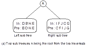
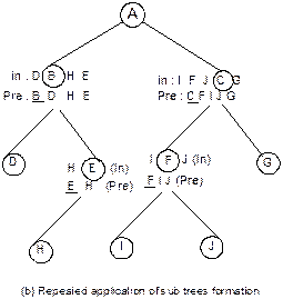

Fig. 8.23 Formation of binary tree from
its inorder and preorder traversals.
Example 8.2: Following is the inorder and postorder
traversals of a binary tree:
Inorder
n1 n2
n3 n4
n5 n6
n7 n8
n9
Postorder
n1 n3
n5 n4
n2 n8
n7 n9
n6
We are to draw the corresponding binary tree.
Construction of binary tree is shown in Figure 8.24.

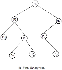
Fig. 8.24 Construction of binary tree
from its inorder and postorder traversals.
Now,
let us define the procedure to construct a binary tree when its two essential
traversals are known. Following is the algorithm InPreTree to form a binary tree from its inorder and preorder
traversals. Let us assume that two traversals are stored in two arrays IN and PRE where the number of nodes is N. The algorithm given
below is a recursive definition. The initial values for the recursion call are I1 = 1, I2 = N, P1 = 1, P2 = N are pointers to
the root node. Figure 8.25 will help to understand the above recursive
definition:
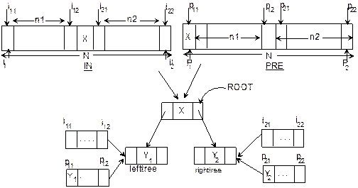
Fig. 8.25 Recursive approach of constructing
a binary tree from inorder and preorder traversals.
Merging
of Two Binary Trees
Another fundamental operation that is possible is
the merge operation. This operation is applicable for trees which are
represented using linked structure. There are two ways that this operation can
be carried out.
Suppose,
T1 and T2 are two binary trees. T2 can be merged with T1 if all the nodes from T2, one by one, is inserted
into the binary tree T1 (insertion may be as internal node when it has to
maintain certain property or may be as external nodes).
Another
way, when the entire tree T2 (or T1) is included as a sub-tree of T1 (or T2). For this, obviously we
need that in either (or both) tree there must be at least one null sub-tree. We
will consider in our subsequent discussion, this second case of merging.
Before,
going to perform the merging, we have to test for compatibility. If in both the
trees, root node have both the left and right sub-trees then merge will fail;
otherwise if T1 has left sub-tree (or right
sub-tree) empty then T2 will be added as the left sub-tree (or right
sub-tree) of the T1
and vice versa. For example, as in Figure 8.27, T1 has right sub-tree empty
hence T2 is added as the right
sub-tree of T1. Note that if T(N)
denotes the number of nodes n in tree T then
T(n1 + n2) = T1(n1) + T2(n2)
where T is the resultant tree of merging T1 and T2.
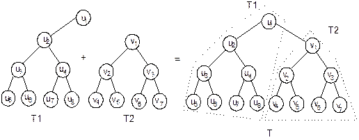
Fig. 8.27 Merging of two binary trees.
Following is the algorithm MERGE to
define the merge operation.
Algorithm MergeTrees
Input: Two pointers ROOT1 and ROOT2 are the roots of the two
binary tree T1 and T2, respectively with
linked
structure.
Output: A binary tree
containing all the nodes of T1 and T2 having pointer to the root as ROOT.
Data structure: Linked structure of
binary trees are considered.
Steps:
|
1. |
If (ROOT1 = NULL)
then // If T1
is empty then T2 is the result |
||||||
|
2. |
|
ROOT
= ROOT2 // Tree T2
is the result |
|||||
|
3. |
|
Exit |
|||||
|
4. |
Else |
||||||
|
5. |
|
If (ROOT2 = NULL)
then // If T2
is empty then T1 is a result |
|||||
|
6. |
|
|
ROOT
= ROOT1 |
||||
|
7. |
|
|
Exit |
||||
|
8. |
|
Else // If both trees are non
empty |
|||||
|
9. |
|
|
If (ROOT1→LCHILD = NULL) then |
||||
|
10. |
|
|
|
ROOT1→LCHILD = ROOT2 // Merge T2 as
the left child of T1 |
|||
|
11. |
|
|
|
ROOT
= ROOT1 |
|||
|
12. |
|
|
Else |
||||
|
13. |
|
|
|
If (ROOT1→RCHILD = NULL) then |
|||
|
14. |
|
|
|
|
ROOT1→RCHILD
= ROOT2 //
Merge T2 as the right child of T1 |
||
|
15. |
|
|
|
|
ROOT
= ROOT1 |
||
|
16. |
|
|
|
Else |
|||
|
17. |
|
|
|
|
If (ROOT2→LCHILD = NULL) then |
||
|
18. |
|
|
|
|
|
ROOT2→LCHILD = ROOT1 // Merge T1 as the
left child of T2 |
|
|
19. |
|
|
|
|
|
ROOT
= ROOT2 |
|
|
20. |
|
|
|
|
Else |
||
|
21. |
|
|
|
|
|
If (ROOT2→RCHILD = NULL) then |
|
|
22. |
|
|
|
|
|
|
ROOT2→RCHILD = ROOT1 // Merge T1 as the right child
of T2 |
|
23. |
|
|
|
|
|
|
ROOT
= ROOT2 |
|
24. |
|
|
|
|
|
Else |
|
|
25. |
|
|
|
|
|
|
Print “Trees are not compatible
for merge operation” |
|
26. |
|
|
|
|
|
|
Exit |
|
27. |
|
|
|
|
|
EndIf |
|
|
28. |
|
|
|
|
EndIf |
||
|
29. |
|
|
|
EndIf |
|||
|
30. |
|
|
EndIf |
||||
|
31. |
|
EndIf |
|||||
|
32. |
EndIf |
||||||
|
33. |
Stop |
||||||
tYPES OF
Binary Trees
There are several types of binary trees possible each with its own properties. Few important and frequently used trees are listed as below.
1. Binary search tree
2. Heap tree
3. Height balanced tree (also known as AVL tree
4. Huffman tree
Binary
Search Tree
A binary tree T is termed as binary search
tree (or binary sorted tree) if each node N of T
satisfies the following property:
The
value at N is greater than every value in the left sub-tree of N
and is less than every value in the right sub-tree of N.
Figure 8.28
shows two binary search trees for two different types of data.
Observe that in Figure 8.28(b), the lexicographical
ordering is taken among the data whereas in Figure 8.31(a), numerical ordering
is taken.
Now,
let us discuss the possible operations on any binary search tree. Operations
those are generally encountered to manipulate this data structures are:
Ÿ Searching for a data
Ÿ Inserting any data into it
Ÿ Deleting any data from it
Ÿ Traversing the tree.
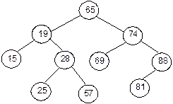
(a)
A Binary search tree with numeric data
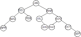
(b)
A Binary search tree with alphabetic data
Fig. 8.28 Binary search trees.
Searching in a binary search tree
Searching for a data in a binary search tree
is much faster than in arrays or linked lists. This is why, in the applications
where frequent searching operations are to be performed, this data structure is
used to store data. In this section, we will discuss how this operation can be
defined.
Suppose,
in a binary search tree T, ITEM be the item of search. We will assume
that, the tree is represented using linked structure.
We
start from the root node R. Then, if ITEM is less than the value in the
root node R, we proceed to its left child; if ITEM is greater than the
value in the node R, we proceed to its right child. The process will be
continued till the ITEM is not found or we reach to a dead end, that is, leave
node. Figure 8.29 shows the track (in shaded line) for searching of 54 in a
binary search tree.
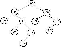
Fig. 8.29 Searching of 54 in a
binary search tree.
The
algorithm for searching an element in a binary search tree is stated as below:
Algorithm Search_BST
Input: ITEM is the data that has to be
searched.
Output: If found then pointer to the node
containing as data ITEM else a message.
Data structure: Linked structure of the binary
tree. Pointer to the root node is ROOT.
Steps:
|
1. |
ptr = ROOT, flag = FALSE // Start from
root |
||
|
2. |
While (ptr ¹
NULL) and
(flag = FALSE) do |
||
|
3. |
|
Case: ITEM < ptr→DATA // Go to the left sub-tree |
|
|
4. |
|
|
ptr = ptr→LCHILD |
|
5. |
|
Case: ptr→DATA = ITEM // Search is successful |
|
|
6. |
|
|
flag = TRUE |
|
7. |
|
Case: ITEM > ptr→ DATA // Go to the right sub-tree |
|
|
8. |
|
|
ptr = ptr→RCHILD |
|
9. |
|
EndCase |
|
|
10. |
EndWhile |
||
|
11. |
If (flag = TRUE) then
// Search is successful |
||
|
12. |
|
Print “ITEM has found at the node”, ptr |
|
|
13. |
Else |
||
|
14. |
|
Print “ITEM does not exist: Search is
unsuccessful” |
|
|
15. |
EndIf |
||
|
16. |
Stop |
||
Inserting into a binary search tree
Insertion operation on a binary search tree is conceptually
very simple. It is in fact, one step more than the searching operation. To
insert a node with data, say ITEM, into a tree, the tree is to be searched
starting from the root node. If ITEM is found, do nothing, otherwise ITEM is to
be inserted at the dead end where search halts. Figure 7.33 shows the insertion
of 5 into a binary tree. Here, search proceeds starting from root node as 6–2–4
then halts when it finds that right child is null (dead end). This simply means
that if 5 occur, then it should occurred in the right part of the node 4. So, 5
should be inserted as the right child of 4.
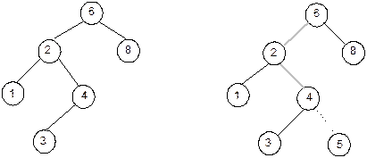
(a) Before insertion (b) Search find the location
where 5 should
be
inserted
Fig. 8.30 Inserting 5 into a binary search tree.
Algorithm
for performing the insertion operation is stated as below:
Algorithm Insert_BST
Input: ITEM is the data component of a node
that has to be inserted.
Output: If there is no node having data ITEM, it
is inserted into the tree else a message.
Data structure: Linked structure of binary tree.
Pointer to the root node is ROOT.
Steps:
|
1. |
ptr
= ROOT, flag = FALSE // Start from
root node |
||
|
2. |
While (ptr ¹ NULL) and (flag = FALSE) do |
||
|
3. |
|
Case: ITEM < ptr→DATA // Go to the left
sub-tree |
|
|
4. |
|
|
ptr1
= ptr |
|
5. |
|
|
ptr
= ptr→LCHILD |
|
6. |
|
Case: ITEM > ptr→DATA // Go to the right
sub-tree |
|
|
7. |
|
|
ptr1
= ptr |
|
8. |
|
|
ptr
= ptr→RCHILD |
|
9. |
|
Case: ptr→DATA = ITEM // Node
exists |
|
|
10. |
|
|
flag
= TRUE |
|
11. |
|
|
Print “ITEM already exists” |
|
12. |
|
|
Exit // Quit
the execution |
|
13. |
|
EndCase |
|
|
14. |
EndWhile |
||
|
16. |
If (ptr = NULL) then // Insert when search halts at dead
end |
||
|
17. |
|
new
= GetNode(NODE) |
|
|
18. |
|
new→DATA = ITEM // Avail a node and then
initialize it |
|
|
19. |
|
new→LCHILD = NULL |
|
|
20. |
|
new→RCHILD = NULL |
|
|
21. |
|
If (ptr1→DATA < ITEM) then // Insert as the right child |
|
|
22. |
|
|
ptr1→RCHILD = new |
|
23. |
|
Else |
|
|
24. |
|
|
ptr1→LCHILD = new // Insert as the
left child |
|
25. |
|
EndIf |
|
|
26. |
EndIf |
||
|
27. |
Stop |
||
Deleting a node from a binary search tree
Another frequently used operations on a binary
search tree is to delete any node from it. This operation, however, is
slightly complicated than the previous two operations discussed.
Suppose
T is a binary search tree, and ITEM is the information given which has
to be deleted from T if it exists in the tree. Suppose N be the
node which contains the information ITEM. Let us assume PARENT(N)
denotes the parent node of N and SUCC(N) denotes the inorder
successor of the node N (inorder successor means the node which
comes after N during the inorder traversal of T). Then the
deletion of the node N depends on the number of its children. Hence,
three cases may arise:
Case 1: N is the leave node
Case 2: N has exactly one child
Case 3: N has two childs
Deletion of N then can be carried out on the
various situations as illustrated in Figure 8.31 and also stated below:
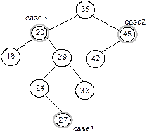
Fig. 8.31 Three cases for deleting a
node N.
Case 1: N is deleted from T by
simply setting the pointer of N in the parent node PARENT(N) by
NULL value. See Figure 8.32(a).
Case 2: N is deleted from T by
simply replacing the pointer of N in PARENT(N) by the pointer of
the only child of N. See the Figure 8.32(b).
Case 3: N is deleted from T by
first deleting SUCC(N) from T (by using Case 1 or Case 2; (it can
be verified that SUCC(N) never has a left child) and then replace the
data content in node N by the data content in node SUCC(N). See
Figure 8.32(c).
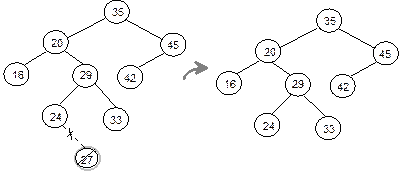
1.
Deletion of the node 27

2.
Deletion of the node 45
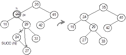
(c) Deletion of the
node 20
Fig.
8.32 Various
cases of deletion in a binary search tree.
Now let us describe the algorithm to delete a node
from a binary search tree.
Algorithm Delete_BST
Input: ITEM is the data of the node to be
deleted.
Output: If the node with data as ITEM exist it
is deleted else a message.
Data structure: Linked structure of binary tree.
Pointer to the root node is ROOT.
Steps:
|
1. |
ptr
= ROOT, flag = FALSE |
||||
|
2. |
While (ptr ¹ NULL) and (flag = FALSE) do // Step to find the
location of the node |
||||
|
3. |
|
Case: ITEM < ptr→DATA |
|||
|
4. |
|
|
parent
= ptr |
||
|
5. |
|
|
ptr
= ptr→LCHILD |
||
|
6. |
|
Case: ITEM > ptr→DATA |
|||
|
7. |
|
|
parent
= ptr |
||
|
8. |
|
|
ptr
= ptr→RCHILD |
||
|
9. |
|
Case: ptr→DATA = ITEM |
|||
|
10. |
|
|
flag
= TRUE |
||
|
11. |
|
EndCase |
|||
|
12. |
EndWhile |
||||
|
13. |
If (flag = FALSE) then
// When the
node does not exist |
||||
|
14. |
|
Print “ITEM does not exist: No
deletion” |
|||
|
15. |
|
Exit // Quit the execution |
|||
|
16. |
EndIf |
||||
|
|
/* DECIDE THE CASE OF DELETION */ |
||||
|
17. |
If (ptr→LCHILD = NULL) and (ptr→RCHILD = NULL) then // Node has no child |
||||
|
18. |
|
case
= 1 |
|||
|
19. |
Else |
||||
|
20. |
|
If (ptr→LCHILD ¹ NULL) and (ptr→RCHILD ¹ NULL) then
// Node contains both the
child |
|||
|
21. |
|
|
case
= 3 |
||
|
22. |
|
Else
// Node contains only one
child |
|||
|
23. |
|
|
case
= 2 |
||
|
24. |
|
EndIf |
|||
|
25. |
EndIf |
||||
|
|
/* DELETION: CASE 1 */ |
||||
|
26. |
If (case = 1) then |
||||
|
27. |
|
If (parent→LCHILD = ptr) then // If the node is a left
child |
|||
|
28 |
|
|
parent→LCHILD = NULL // Set pointer of its
parent |
||
|
29. |
|
Else |
|||
|
30. |
|
|
parent→RCHILD = NULL |
||
|
31. |
|
EndIf |
|||
|
32. |
|
ReturnNode(ptr) // Return deleted node to
the memory bank |
|||
|
33. |
EndIf |
||||
|
|
/*
DELETION: CASE 2 */ |
||||
|
34. |
If (case = 2) then // When the node
contains only one child |
||||
|
35. |
|
If (parent→LCHILD = ptr) then // If the node
is a left child |
|||
|
36. |
|
|
If (ptr→LCHILD = NULL) then |
||
|
37. |
|
|
|
parent→LCHILD = ptr→RCHILD |
|
|
38. |
|
|
Else |
||
|
39. |
|
|
|
parent→LCHILD = ptr→LCHILD |
|
|
40. |
|
|
EndIf |
||
|
41. |
|
Else |
|||
|
42. |
|
|
If (parent→RCHILD = ptr) then |
||
|
43. |
|
|
|
If (ptr→LCHILD = NULL) then |
|
|
44. |
|
|
|
|
parent→RCHILD = ptr→RCHILD |
|
45. |
|
|
|
Else |
|
|
46. |
|
|
|
|
parent→RCHILD = ptr→LCHILD |
|
47. |
|
|
|
EndIf |
|
|
48. |
|
|
EndIf |
||
|
49. |
|
EndIf |
|||
|
50. |
|
ReturmnNode(ptr) // Return deleted node to the memory
bank |
|||
|
51. |
EndIf |
||||
|
|
/*
DELETION: CASE 3 */ |
||||
|
52. |
If (case = 3)
// When contains both child |
||||
|
53. |
|
ptr1
= SUCC(ptr) // Find the in order
successor of the node |
|||
|
54. |
|
item1
= ptr1→DATA |
|||
|
55. |
|
Delete_BST (item1)
// Delete the inorder successor |
|||
|
56. |
|
ptr→DATA = item1 // Replace the
data with the data of in order successor |
|||
|
57. |
EndIf |
||||
|
58. |
Stop |
||||
Note that, we assume the function SUCC(ptr)
which returns pointer to the inorder successor of the node ptr. It can be verified that
inorder successor of ptr always occurs in the right
sub-tree of ptr, and inorder successor of ptr does not have left child.
Figure 8.33 shows an instance.
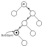
Fig. 8.33 Inorder successor of a node
ptr.
Finding
the inorder successor of any node is very easy and is stated as below:
Algorithm SUCC
Input: Pointer to a node PTR whose inorder
successor is to be known.
Output: Pointer to the inorder successor of ptr.
Data structure: Linked structure of binary tree.
Steps:
|
1. |
ptr1 = PTR→RCHILD // Move to the right sub-tree |
||
|
2. |
If (ptr1 ¹ NULL) then // If right sub-tree is not empty |
||
|
3. |
|
While (ptr1→LCHILD ¹ NULL) do // Move to the left-most
end |
|
|
4. |
|
|
ptr1 = ptr1→LCHILD |
|
5. |
|
EndWhile |
|
|
6. |
EndIf |
||
|
7. |
Return(ptr1)
// Return the pointer of the inorder
successor |
||
|
8. |
Stop |
||
Traversals on binary search tree
All the traversal operations are applicable in
binary search trees without any alteration. It can be verified that inorder traversal
on a binary search tree will give the sorted order of data in ascending order.
If we require to sort a set of data, a binary search tree can be built with
those data and then inorder traversal can be applied. This method of sorting is
known as binary sort and this is why binary search tree is also termed
as binary sorted tree. This sorting method is considered as one of the
efficient sorting method.
Application of binary search trees
Binary
search tree is one of the most important data structure and it has a large
number of applications. It can be used in sorting method and in searching
method. In fact, binary search tree is used to define other data structure, for
example, B tree. Here, we shall learn an example of it in the context of
searching when the key values are not necessarily equally likely. In other
words, there are several applications where key values are accessed according
to some frequency values. One such application, suppose, writing a translator
from English to Hindi. Here, for each occurrence of each English word in the
input text we are to look up its Hindi equivalent. One simple solution to this
problem is to construct a binary search tree for all words involved in the
English vocabulary. With this solution it may be the case that a frequently
used word such as “the” appears far from the root while a rarely used word such
as “neanderthal” appears near the root. This is obviously not a good a way of
organizing the binary search tree because it effectively slows down the
translation process. This consideration makes it natural to ask about the best
possible tree for searching a table of keys with given frequencies.
Heap
Trees
Suppose, H is a complete binary tree. Then it will
be termed as heap tree, if it satisfies the following properties:
(i) For each node N in H, the value at N is greater than or equal to the value of each of the children of N.
(ii) Or in other words, N has the value which is greater than or equal to the value of every successor of N.
Such a heap tree is called max heap. Similarly, min heap is possible, where any node N has the value less than or equal to the value of any of the successors of N. Figure 8.34 shows max heap and min heap with numeric data:
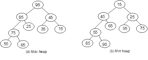
Fig. 8.34 Heap trees.
Note that in a max heap, the root node contains the largest data whereas in a min heap it contains the smallest data.
Representation of heap tree
A heap tree can be represented using linked structure. But single array representation has certain advantages for a heap tree over its linked representation. As heap tree is a complete binary tree, so there will be no wastage of array space between two non-null entries; if any null entries, these are only at the tail of the array. Another facility is that we do not have to maintain any links of descendants (child), here, these are automatically implied, to access a child only a few simple arithmetic computations are involved. The major advantage with this representation is that, from a node we can go in both directions, towards its ancestors and towards its successor. This is, although possible in linked structure but is a matter of maintenance of extra link field.
Hence, for a heap tree, it is better to consider the single array representation. Figure 8.35 shows a heap tree (as represented in Figure 8.34(b)) using a single array.

Fig. 8.35 Single array
representation of a heap (min) tree.
During the subsequent discussions on heap tree we will assume the single array representation unless we specify the other.
Operations on heap tree
The major operations required to be performed on a heap tree are: insertion, deletion and merging. Let us discuss all these operations one by one.
Insertion
into a heap tree
This
operation is used to insert a node into an existing heap tree satisfying the
properties of heap tree. Repeated insertions of data, starting from an empty
heap tree, one can build up a heap tree. Let us first discuss the method of
insertion, then formal description of the procedure will be described.
Let us consider the heap (max) tree as shown in Figure 8.36. We want to insert 19 and 111 in it. The principle of insertion is that, first we have to adjoin the data in the complete binary tree. Next, we have to compare it with the data in its parent; if the value is greater than that at parent then interchange the values. This will continue between two nodes on path from the newly inserted node to the root node till we get a parent whose value is greater than its child or we reached at the root.
For illustration, 19 is added as the left child of 25, Figure 7.36(b). Its value is compared with its parent’s value, and to be a max heap, parent’s value > child’s value is satisfied, hence interchange as well as further comparison is no more required.
As an another illustration, let us consider the case of inserting 111 into the resultant heap tree. First, 111 will be added as right child of 25, when 111 is compared with 25 it requires interchange. Next, 111 is compared with 85, another interchange takes place. At the last, 111 is compared with 95 and then another interchange occurs. Now, our process stops here, as 111 is now in root node. The path on which these comparisons and interchanges have taken places are shown by dashed line, Figure 8.36(c).
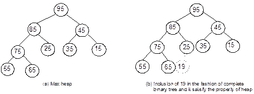

Fig. 8.36 Insertion of 19 and 111 into a heap tree.
Now, we are in a position to describe the algorithm InsertMaxHeap to insert a data into a max heap tree. Let us assume that A[1...SIZE] be an array of data where the heap tree is stored and its maximum capacity is SIZE. N denotes the number of nodes currently in the heap tree. For an empty heap tree, N = 0.
Algorithm InsertMaxHeap
Input: ITEM, the data to be inserted; N, the strength of nodes.
Output: ITEM is inserted into the heap tree.
Data structure: Array A[1...SIZE] stores the heap tree; N being the number of node in the tree.
Steps:
|
1. |
If (N ³
SIZE) then |
||
|
2. |
|
Print “Heap tree is
saturated: Insertion is void” |
|
|
3. |
|
Exit |
|
|
4. |
Else |
||
|
5. |
|
N = N + 1 |
|
|
6. |
|
A[N] = ITEM // Adjoin the data in the complete
binary tree |
|
|
7. |
|
i = N // Last node is the current node |
|
|
8. |
|
p = i div 2. // Its parent node is at p |
|
|
9. |
|
While (p > 0) and (A[p] < A[i])
do // Continue till the root is reached or
out of order |
|
|
10. |
|
|
temp
= A[i] |
|
11. |
|
|
A[i] = A[p] |
|
12. |
|
|
A[p] = temp |
|
13. |
|
|
i = p // Parent becomes child |
|
14. |
|
|
p = p div 2 // Parent of parent becomes new
parent |
|
15. |
|
EndWhile |
|
|
16. |
EndIf |
||
|
17. |
Stop |
||
Deletion
of a node from heap tree
Any
node can be deleted from a heap tree. But from the application point of view,
deleting the root node has some special importance. We will first illustrate
the principle of such deletion and then the formal description. The principle
can be stated as below:
· Read the root node into a temporary storage say, ITEM.
· Replace the root node by the last node in the heap tree. Then reheap the tree as stated below:
— Let newly
modified root node be the current node. Compare its value with the value of its
two child. Let X be the child whose value is the largest. Interchange
the value of X with the value of the current node.
— Make X as the current node.
— Continue reheap, if the current node is not an empty node.
This is illustrated as in Figure 8.37. In Fig. 8.37, the root node is 99. The last node is 26, and it is in the level 3. So, 99 is replaced by 26 and this node with data 26 is removed from the tree. Next 26 at root node is compared with its two child 45 and 63. As 63 is greater, so they are interchanged. Now, 26 is compared with its children, namely, 57 and 42, as 57 is greater, so they are interchanged. Now, 26 appears as the leave node, hence reheap is completed.

Fig. 8.37 Deletion of the
root node 99 from a max heap tree.
The algorithm for the deletion of a node from a heap (max) tree is is given below:
Algorithm MaxHeapdelete
Input: A heap tree with elements.
Output: ITEM is being the data deleted and the remaining tree after deletion.
Data structures: An array A[1... SIZE] storing the heap tree; N is the number of nodes.
Steps:
|
1. |
If (N = 0) then |
||||
|
2. |
|
Print “Heap tree is
exhausted: Deletion is not possible” |
|||
|
3. |
|
Exit |
|||
|
4. |
EndIf |
||||
|
5. |
ITEM
= A[1] // Value at the root node
under deletion |
||||
|
6. |
A[1] = A[N] // Replace the value at root by its counterpart at last node on last level |
||||
|
7. |
N = N – 1 // Size of the heap tree
is reduced by 1 |
||||
|
8. |
flag
= FALSE, i = 1 |
||||
|
9. |
While(flag = FALSE) and (i < N) do // Rebuild
the heap tree |
||||
|
10. |
|
lchild = 2 * i, rchild = 2 * i+1 // Addresses of left and right child of the current node |
|||
|
11. |
|
If (lchild £ N) then |
|||
|
12. |
|
|
x = A[lchild] |
||
|
13. |
|
Else |
|||
|
14. |
|
|
x
= – ¥ |
||
|
15. |
|
EndIf |
|||
|
16. |
|
If (rchild £ N) then |
|||
|
17. |
|
|
y = A[rchild] |
||
|
18. |
|
Else |
|||
|
19. |
|
|
y
= – ¥ |
||
|
20. |
|
EndIf |
|||
|
21. |
|
If (A[i] > x)
and (A[i] > y) then // If parent is larger than
its child |
|||
|
22. |
|
|
flag
= TRUE // Reheap
is over |
||
|
23. |
|
Else // Any child may have
large value |
|||
|
24. |
|
|
If (x > y) and (A[i] < x) // If left child is larger than right child |
||
|
25. |
|
|
|
Swap(A[i], A[lchild]) // Interchange the data between parent and left child |
|
|
26. |
|
|
|
i = lchild // Left child becomes the current node |
|
|
27. |
|
|
Else |
||
|
28. |
|
|
|
If (y > x) and (A[i] < y) // If right child is larger than left child |
|
|
29. |
|
|
|
|
Swap(A[i], A[rchild]) //Interchange the data between parent and right child |
|
30. |
|
|
|
|
i = rchild // Right child becomes the current node |
|
31. |
|
|
|
EndIf |
|
|
32. |
|
|
EndIf |
||
|
33. |
|
EndIf |
|||
|
34. |
EndWhile |
||||
|
35. |
Stop |
||||
Merging
two heap trees
Consider,
two heap trees H1
and H2. Merging the tree H2 with H1 means to include all the
nodes from H2 to H1. H2 may be min heap or max heap
and the resultant tree will be min heap if H1 is min heap else it will be
max heap.
Merging operation consists of two steps: Continue steps 1 and 2 while H2 is not empty:
1. Delete the root node, say x, from H2.
2. Insert the node x into H1 satisfying the property of H1.
Figure 8.38 illustrates the merge operation between two heap trees.
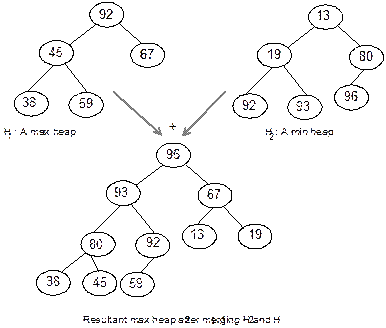
Fig. 8.38 Merging two
heap trees.
Application of heap trees
There are two main applications of heap trees known: (a) sorting and (b) priority queue implementation. The sorting method which is based on heap tree is called heap sort and known as the efficient sorting method. We have mentioned the problem of implementing priority queues using linked structure; using heap tree there is an elegant solution possible for the same problem. Let us discuss briefly about each application.
Sorting
using heap tree
Any
kind of data can be sorted either in ascending order or in descending order
using heap tree. This actually comprises of the following steps:
Step 1: Build a heap tree with the given set of data.
Step 2: (a) Delete the root node from the heap.
(b) Rebuild the heap after the deletion.
(c) Place the deleted node in the output.
Step 3: Continue Step 2 until the heap tree is empty.
It can be noted that, to sort the data in ascending (descending) order, we have to built max heap (min heap) in Step 1. In order to trace the method, let us assume the case of sorting the following set of data in ascending order:
33, 14, 65, 02, 76, 69, 59, 85, 47, 99, 98
As per Step 1, first we have to built the max heap tree which can be done as below: Successively remove an element from the list and insert it into the heap starting from an empty heap. This results the heap tree as shown in Figure 8.39(a).
We do not require another array to store the output, instead, in the same array where the heap is stored. Following Step 2, let us see, how the sorted array will grow gradually.
99 is deleted and it is replaced by 76, the last node in the heap; the currently deleted node is placed in the position of 76, the last node. Now, the last node is 14. This is simply swapping the root node and the last node and shifting pointer to the last node just once towards the left. This is illustrated in Figure 8.39(b).
Next, we are to rebuild the heap tree. This is as illustrated as in Figure 8.39(c)–(d).

(a)
A Heap tree from a given set of data
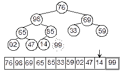
(b)
Swaping the root and the last node

(c)
Rebuild the heap tree

(d)
Continuation of step 2 after selecting 98
![]()
(e)
Sorted list when the heap is empty
Fig. 8.39(a)–(e) Tracing of
heap sort.
The algorithm HeapSort is presented below to implement the sorting method.
Algorithm HeapSort
Input: A set of N input data.
Output: Sorted data in ascending order.
Data structure: An array A where the data will be stored.
Steps:
|
1. |
BuildMaxHeap(A) // To create the heap H from the set of data |
||||
|
2. |
i = N |
||||
|
3. |
While (i > 1) do // Continue until heap contains single element |
||||
|
4. |
|
Swap (A[1], A[i]) // Delete the root node and replace it by the last node |
|||
|
5. |
|
i = i – 1 // Pointer to the last node shifted towards the left |
|||
|
6. |
|
j = 1 // To rebuild the heap |
|||
|
7. |
|
While (j < i) do |
|||
|
8. |
|
|
lchild = 2 * j // Left child |
||
|
9. |
|
|
rchild = 2 * j + 1 // Right child |
||
|
10. |
|
|
If (A[j] < A[lchild]) and (A[lchild] > A[rchild]) then |
||
|
11. |
|
|
|
Swap(A[j], A[lchild]) |
|
|
12. |
|
|
|
j = lchild |
|
|
13. |
|
|
Else |
||
|
14. |
|
|
|
If (A[j] < A[rchild]) and (A[rchild] > A[lchild]) then |
|
|
15. |
|
|
|
|
Swap(A[j], A[rchild]) |
|
16. |
|
|
|
|
j = rchild |
|
17. |
|
|
|
Else |
|
|
18. |
|
|
|
|
Break( ) // Rebuild is completed: break the loop |
|
19. |
|
|
|
EndIf |
|
|
20. |
|
|
EndIf |
||
|
21. |
|
EndWhile |
|||
|
22. |
EndWhile |
||||
|
23. |
Stop |
||||
In the above algorithm, we assume a procedure BuildMaxHeap to build a heap from a given set of data, which is nothing but the repeated insertions into the heap starting from an empty heap using the procedure MaxHeapInsert. Other procedure, like Swap(...), bears the usual meaning.
Priority queue implementation using heap tree
A priority queue can be implemented using circular array, linked list, etc. Another simplified implementation is possible using heap tree; the heap, however, can be represented using an array. This implementation is therefore free from the complexities of circular array and linked list but getting the advantages of simplicities of array.
It may be
recalled that, heap trees allow the duplicity of data in it. Elements
associated
with their priority values are to be stored in the form of heap tree, which can
be formed based on their priority values. The top priority element that has to
be processed first is at the root; so it can be deleted and heap can be rebuilt
to get the next element to be processed, and so on.
As an illustration, consider the following processes with their priorities:
Process P1 P2 P3 P4 P5 P6 P7 P8 P9 P10
Priority 5 4 3 4 5 5 3 2 1 5
These processes enter the system in the order as listed above at time 0, say. Assume that a process having higher priority value will be serviced first. The heap tree that can be formed considering the process’ priority values is shown in Figure 8.40(a).
The order of servicing the processes are successive deletion of roots from the heap as illustrated in Figures 8.40(b)–(j).
Refer to Figures 8.40(b), (c), (e), we note that out of two processes, having the same priority and in the same level, that process climbed to the root which precedes the other in their order of arrival. So, the processes are served in the sequence as
P1 P5 P6 P10 P2 P4 P3 P7 P8 P9
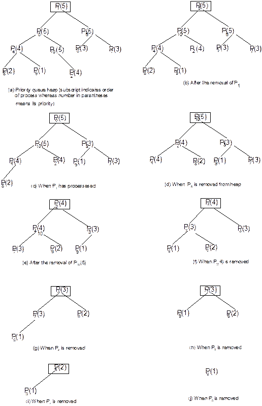
Fig. 8.40 Priority
queue implementation using a heap tree.
Height
Balanced Binary Tree
Let us consider the following set of data:
jan, feb, mar, apr, may, jun, jul, aug, sep, oct, nov, dec
We know that for a given set of data binary search tree is not necessarily unique. In other words, structure of a binary search tree depends on the ordering of data in the input. Hence, for the above mentioned data there are 12! binary search trees possible (each corresponding to an arrangement in the permutation of data). Only six of them are presented as shown in Figure 8.41.
Next, let us define the average search time G, for an element in a binary search tree as

where
ti = Number of comparisons for the i-th element
n = Total number of elements in the binary search tree
Thus with
this, the average search time G for the binary search trees as mentioned in
Figure 7.52 can be calculated as:
G(a) = 6.50 G(b) = 4.00
G(c) = 3.50 G(d) = 3.08
G(e) = 3.08 G(f) = 3.16
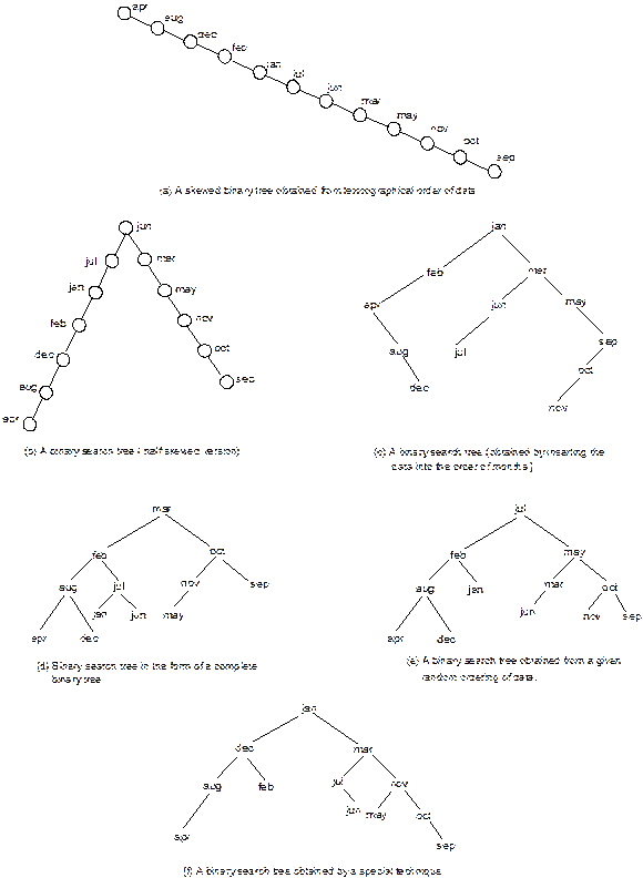
Figure 8.41(a)–(f) Six examples
of binary search trees from a given set of data.
From this calculation, it is evident that, out of six varieties of representations, last three representations are efficient from the searching time point of view. The worst representation is the skewed form of the binary search tree, which needs the highest average search time.
Now, here the question arises is that for a given set of data how a binary search tree can be constructed so that it will involve minimum average search time. The answer lies in the concept of height balanced binary search tree. A binary search tree can be made by means of calculating the balance factor of each node. We first define the term balance factor first. The balance factor of a binary tree (bf) is defined as
bf = Height of the left sub-tree (hL) – Height of the right sub-tree (hR)
Height (h) of a binary tree as mentioned earlier is
h = Number of nodes visited in traversing a branch which leads to a leaf node at the deepest level of the tree.
Definition. A binary search tree is said to be height balanced binary search tree if all its nodes have a balance factor of 1, 0 or –1. That is,
|bf| = |hL – hR| £ 1
for every node in the tree.
For example, Figure 8.42 represents two binary search trees out of which one satisfies the properties of height balanced binary tree and other does not.

Fig. 8.42 Two binary
search trees with the balance factors of each node.
It can be noted that a height balanced binary tree is always a binary search tree and a complete binary search tree is always height balanced, but the reverse may not be true.
The basic objective of the height balanced binary search tree is to perform the searching, insertion and deletion operations efficiently. These operations may not be with the minimum time but less than that of in unbalanced binary search tree. It can be realized that the search time in case of complete binary search tree is minimum but insertion and deletion may not be with minimum time always.
In the following discussion, we will see how an unbalanced binary search tree can be converted into a height balanced binary search tree. Suppose, initially there is a height balanced binary tree. Whenever a new node is inserted into it (or deleted from it), it may become unbalanced. We will first see the mechanism to balance an unbalance tree due to insertion of a node.
Following steps are to be adopted.
1. Insert node into a binary search tree: Insert the node into its proper position following the properties of binary search tree.
2. Compute the balance factors: On the path starting from the root node to the node newly inserted, compute the balance factors of each node. It can be verified that change in balance factors will occur only in this path.
3. Decide the pivot node: On the path as traced in Step 2, determine whether the absolute value of any node’s balance factor is switched from 1 to 2. If so, the tree becomes unbalanced. The node whose absolute value of balance factor is switched from 1 to 2, mark it as a special node called pivot node. (There may be more than one node whose balance factor |bf| is switched from 1 to 2 but the nearest node to newly inserted node will be the pivot node.)
4. Balance the unbalance tree: It is necessary to manipulate pointers centred at the pivot node to bring the tree back into height balance. This pointer manipulation is well known as AVL rotation, mechanism of which is illustrated next in the text.
AVL rotations
In order to balance a tree, one elegant method devised in 1962 by two Russian mathematicians, G.M. Adelson-Velskii and E.M. Lendis, and the method is named as AVL rotation in their honour.
There are four cases of rotations possible which is discussed as below:
Case 1: Unbalance
occurred due to the insertion in the left sub-tree of the left child of the
pivot node.
Figure 8.43 illustrates the rotation for Case 1. In this case, following manipulations in pointers take place:
· Right sub-tree (AR) of left child (A) of pivot node (P) becomes the left sub-tree of P.
· P becomes the right child of A.
· Left sub-tree (AL) of A remains the same.
This case is called LEFT-TO-LEFT insertion.

Fig. 8.43 AVL rotation
when unbalance occurs due to the insertion in the left sub-tree of the
left child of the
pivot node (Left-to-left
insertion).
Illustration. Consider the illustration as shown in Figure 8.44. Node 2 is inserted into the initially heright balances tree (see Figure 8.44(a)). Here, 6 is the pivot node because this is the nearest node from the newly inserted node whose balance factor is switched from 1 to 2 (see Figure 8.44(b)). This insertion corresponds to the case of LEFT-TO-LEFT insertion. AVL rotation required is depicted in Figures 8.44(c)–(d). Final height balanced tree is shown as in Figure 8.44(e) with balance factor of each node.
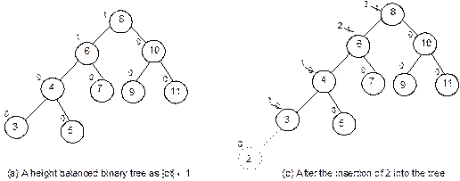
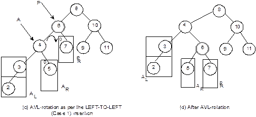
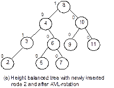
Fig. 8.44(a)–(e) LEFT-to-Left insertion and AVL rotation to
make the tree height balanced.
Case 2: Unbalance occurs due to the insertion in the right sub-tree of the right child of the pivot node. This case is the reverse and symmetric to Case 1. This rotation is illustrated in Figure 8.42. In this case, the following manipulations in pointers take place:
· Left sub-tree (BL) of right child (B) of pivot node (P) becomes the right sub-tree of P.
· P become the left child of B.
· Right sub-tree (BR) of B remains same.
This case is known as RIGHT-TO-RIGHT insertion.
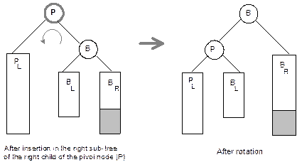
Fig. 8.42 AVL rotation when
unbalance occurs due to insertion in the right sub-tree of the right child of
the pivot node (RIGHT-TO-RIGHT insertion).
Illustration. Case 2 of AVL rotation occurs due to RIGHT-TO-RIGHT insertion. A situation is illustrated in Figure 8.43. Due to the insertion of 12, the tree becomes unbalance (see Figure 8.43(a)) and the pivot node in this case is 9. The unbalance occurs due to the insertion as the right child of the right sub-tree of the pivot node. The rotation required is illustrated in Figure 8.43(b).

Fig. 8.43 RIGHT-TO-RIGHT insertion
and corresponding AVL rotation.
Case 3: Unbalance occurs due to the insertion in the right sub-tree of the left child of the pivot node. Figure 8.44 illustrates the rotation required for this case of insertion. This case is known as LEFT-TO-RIGHT insertion.
Case 3 involves two rotations for the manipulation in pointers:
Rotation 1
· Left sub-tree (BL) of the right child (B) of the left child of the pivot node (P) becomes the right sub-tree of the left child (A).
· Left child (A) of the pivot node (P) becomes the left child of B.
Rotation
2
· Right sub-tree (BR) of the right child (B) of the left child (A) of the PIVOT node (P) becomes the left sub-tree of P.
· P becomes the right child of B.
This case is known as LEFT-TO-RIGHT insertion. If insertion occurs at BR instead of BL, it corresponds to the same as Case 3.

Fig. 8.44 AVL rotation
when unbalance occurs due to the insertion in the right sub-tree of the left
child of the pivot node (LEFT-TO-Right
insertion).
Illustration. Consider the illustration as shown in Figure 8.45 for LEFT-TO-RIGHT insertion and corresponding AVL rotation.

Figure 8.45(a)–(d) LEFT-TO-RIGHT
insertion and AVL rotation.
Case 4: Unbalance occurs due to the insertion in the left sub-tree of right child of the pivot node. This case is the reverse and symmetric to Case 3. This case is known as RIGHT-TO-LEFT insertion. The rotation requires balancing the tree in this situation as illustrated in Figure 8.46.
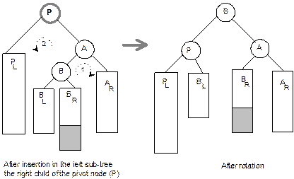
Fig. 8.46 AVL rotation
when unbalance occurs due to the insertion at the left sub-tree of right child
of the pivot node (RIGHT-TO-LEFT insertion).
There are two rotations for the manipulations of pointers in this case, these are:
Rotation 1
· Right sub-tree (BR) of the left child (B) of the right child (A) of the pivot node (P) becomes the left sub-tree of A.
· Right child (A) of the pivot node (P) becomes the right child of B.
Rotation 2
· Left sub-tree (BL) of the right child (B) of the right child (A) of the pivot rode (P) becomes the right sub-tree of P.
· P becomes the left child of B.
This case is known as RIGHT-TO-LEFT insertion. We have considered the insertion in BR; the AVL rotation is same, if the node is inserted in BL.
Illustration. Figure 8.47 illustrates the Case 4 of AVL rotation required during RIGHT-TO-LEFT insertion.

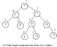
Fig. 8.47(a)–(c) RIGHT-TO-LEFT
insertion and AVL rotation.
Height
of a height balanced binary tree
We
have learned how to create a height balanced binary (AVL) tree. Let us now analyze
on the height of a height balanced binary tree. Let us calculate the maximum
height that an AVL tree may have. To determine the maximum height that an AVL
tree with n nodes have, we first calculate the minimum number of nodes
that an AVL tree of height h can
have.
It
can be proved that the maximum height possible in an AVL tree with n number of nodes is given by
![]()
Weighted Binary Tree
Before discussing about weighted binary tree, let us first introduce the following terms related to the weighted binary tree:
Path length. Path length of a node in a tree is defined as the number of edges that has to be traversed from the node to the root node.
External node. The node with zero children is called an external node (or in other words, an external node is nothing but a leaf node).
Internal node. A node with one or more children is called an internal node.
Refer Figure 8.48, all the internal nodes are drawn as circles and all the external nodes are drawn as squares. Thus, nodes labelled as N1, N2, ..., N9 are internal nodes and that of L1, L2, ..., L10 are external nodes. A binary tree containing such distinctive nodes as external nodes, is known as extended binary tree.
It is already discussed in Section 7.2.2 vide Lemma 8.5 that if NE and NI denote the number of external and internal nodes then NE = NI + 1. It can be verified from Figure 8.48, where NE = 10, NI = 9, and thus NE = NI + 1.

Fig. 8.48 An extended
binary tree.
Path length of a node as defined can be verified from Figure 8.48:
Path length of N1 = 0
Path length of N9 = 4
Path length of L5 = 4
Path length of L8 = 5
and so on. Now, we will define additional two terms: external path length and internal path length.
External path length. External path length (let it be denoted as E) of a binary tree is defined as the sum of all path lengths, summed over each path from the root node of the tree to an external node. Alternatively,
![]()
where, Pi denotes the path length of the i-th external node.
Internal path length. Internal path length (let it be denoted as I) of a binary tree can be defined analogously as the sum of path lengths of all internal nodes in the tree. Alternatively,
![]()
where, Pi denotes the path length of the i-th internal node.
Refer Figure 8.48, whose external path length and internal path length can be computed as
L1 L2 L3 L4 L5 L6 L7 L8 L9 L10
E = 2 + 3 + 3 + 4 + 4 + 3 + 3 + 5 + 5 + 4 = 36
N1 N2 N3 N4 N5 N6 N7 N8 N9
I = 0 + 1 + 2 + 1 + 2 + 3 + 2 + 3 + 4 = 18
There is a relation between the external path length (E) and internal path length (I), which is stated in Lemma 8.8:
|
Lemma 8.8 |
|
|
In a binary tree with n internal nodes, if I denotes the internal path length, then external path length, E = I + 2n. |
|
Proof : This lemma can be proved by the method of induction and is left as an exercise.
The above lemma can be verified from the extended tree as presented in Figure 7.68, where n = 9, E = 36 and I = 18.
Now, let us discuss, for a given number of internal node, say n, what is the minimum and maximum external path lengths possible. It is evident from Lemma 7.13 that binary trees with minimum I also have the minimum E.
It can be easily realized that, a binary tree is having maximum internal path lengths when it is skewed and minimum when all the internal nodes are as close to the root as possible, that is, when it is a complete binary tree (Figure 8.49).
If Imax denotes the maximum internal path length of a binary tree with n internal nodes, then
![]()
Similarly, if Imin denotes the minimum internal path length of a binary tree with n internal nodes, then
![]()
where lmax is the maximum level.

Fig. 8.49 Two binary
trees with minimum and maximum path lengths.
Weighted path length
So far we have discussed about the extended binary trees where the values of internal and external nodes are same and is one unit, say. But the path lengths considering different values of nodes are possible. We will restrict our discussion in case of binary trees where all internal nodes have unit values but each of the external nodes are assigned a (non-negative) number called weights. The external path length with these weights are called external weighted path length (or, simply weighted path length) and the corresponding binary tree is termed as extended weighted binary tree (or, simply weighted binary tree).
Hence, if Wi is a weight of an external node ni and its path length is Li then, weighted path length, P is:
![]() (7.30)
(7.30)
for a binary tree with n external nodes.
Figure 8.50 illustrates a weighted binary tree.

Fig. 8.50 A weighted binary tree
with 7 external nodes.
The weighted external path length (P) of the tree in Figure 8.50 is calculated as below:
P = W1L1+ W2L2 + W3L3 + W4L4 + W5L5 + W6L6 + W7L7
= 2 ´ 2 + 5 ´ 2 + 3 ´ 4 + 4 ´ 4 + 1 ´ 3 + 7 ´ 3 + 6 ´ 3
= 4 + 10 + 12 + 16 + 3 + 21 + 18
= 84
Our next objective is to construct a weighted binary tree for a given set of weights of the external nodes, so that the weighted path length is minimum. As earlier, we have noticed that path lengths are minimum when the extended tree is a complete binary tree, it is not true always in case of weighted binary trees. For an illustration, let us consider four external nodes having weights 2, 3, 5 and 9. Three weighted binary trees are constructed as shown in Figure 8.51.
The weighted path lengths of the trees are:
P(T1) = 2 ´ 2 + 3 ´ 2 + 5 ´ 2 + 9 ´ 2 = 38
P(T2) = 2 ´ 1 + 9 ´ 2 + 5 ´ 3 + 3 ´ 3 = 44
P(T3) = 5 ´ 2 + 2 ´ 3 + 3 ´ 3 + 9 ´ 1 = 34
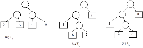
Fig. 8.51 Three
weighted binary trees with 4 weights.
So, here T1, which is in the form of complete binary tree is not a minimum weighted binary tree (a weighted binary tree with minimum external weighted path length may be termed as minimum weighted binary tree), where T3 is a minimum weighted binary tree.
An elegant solution to the problem of finding a binary tree with minimum weighted external path length was given by D. Huffman. The tree that can be constructed with the Huffman’s algorithm is guaranteed to be a minimum weighted binary tree and to honour the inventor, such trees are alternatively termed as Huffman tree. Huffman’s algorithm is an iterative method, which is stated informally as below:
Suppose, we have to construct a minimum weighted binary tree (Huffman tree) with n weights W1, W2, . . ., Wn.
· Sort the weights in ascending order.
· Obtain a sub-tree with two minimum weights as the weights of external nodes.
· Include the weighted path length of the sub-tree so obtained into the list of weights.
· Repeat the procedure until the list contains single weight.
It can be noted that, Huffman’s algorithm constructs the tree from bottom up (starting from the external nodes to the root nodes) rather than from top down.
The algorithm is illustrated with an example as shown in the Figure 8.51. Suppose the following weights are given as input:
External node: A B C D E F
Weight: 2 5 3 4 1 7
The final Huffman tree is shown in Figure 8.51(e). The weighted path length of the tree can easily be obtained by sum up all the values in the internal nodes. Thus, path length of the resultant tree is = 22 + 9 + 13 + 6 + 3 = 53.

Fig. 8.51 Continued.

Fig. 8.51 Construction
of Huffman tree.
There is as an alternative weighted binary tree for the same set of data which can be constructed by trial basis as shown in Figure 8.52. The weighted path length of which can be estimated as
P = 22 + 8 + 14 + 3 + 7 = 54
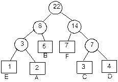
Fig. 8.52 A weighted
binary tree but not Huffman tree.
The above example is included to emphasize the fact that the Huffman tree so obtained as in Figure 8.51 is guaranteed to be a minimum weighted external binary tree. Reader can verify this by obtaining any other weighted binary tree possible.
It can also be noted that construction of Huffman tree by Huffman’s algorithm is not unique. Figure 8.53 represents two Huffman trees obtained by following the Huffman’s algorithm for the same set of weights.
Here, both the trees have the same weighted path length (= 53) and they are Huffman trees, that is, the external weighted binary tree with minimum external path length, although not unique.
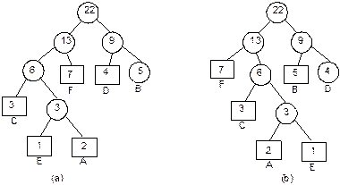
Fig. 8.53 Two minimum
weighted Huffman trees with the same set of weights.
Implementation of Huffman tree
Now let us consider the implementation aspect of Huffman tree. We will assume the node structure as mentioned below for a node to form Huffman tree.
![]()
Here. LCHILD and RCHILD are as usual two link fields, WEIGHT is a numeric field to store the weight of a node in case of external node, and path length of sub-tree taking the current node as the root in case of internal node. DATA is to store the label for a node; for all the internal nodes, DATA component will be empty. Also, we will assume a pointer array PARRAY[. . .] to store the pointers to nodes in a Huffman tree and Sort_PARRAY to sort the PARRAY[. . .] the elements between the array locations I and N (with respect to their weights). The Algorithm BuildHuffmanTree is now given as below:
Algorithm BuildHuffmanTree
Input: W = [W1, W2, ..., WN] is a set of weights of N external nodes.
Output: A Huffman tree having ROOT as the pointer to its root note with the given set of data as the weights of external nodes.
Data structure: Linked structure of Huffman tree.
Steps:
|
1. |
For i = 1 to N do // Read the external nodes and initialize the PARRAY |
|
|
2. |
|
ptr = GetNode(NODE) |
|
3. |
|
ptr→WEIGHT = W[i] // To read the weight for the external node |
|
4. |
|
ptr→LCHILD = NULL // Link fields of external nodes are empty |
|
5. |
|
ptr→RCHILD = NULL |
|
6. |
|
PARRAY[i] = ptr // Store the node into the PARRAY |
|
7. |
EndFor |
|
|
8. |
i = 1 |
|
|
9. |
While (i < N) do |
|
|
10. |
|
Sort_PARRAY(i, N) // Sort the weights from i to N in ascending order |
|
11. |
|
ptr = GetNode(NODE) // Get a node for internal node |
|
12. |
|
ptr→DATA = NULL |
|
13. |
|
ptr→LCHILD = PARRAY[i] // Include the lowest weight as the left sub-tree |
|
14. |
|
ptr→RCHILD = ptr→PARRAY[i + 1] // Include the second lowest weight as the right sub-tree |
|
15. |
|
ptr→WEIGHT = (ptr→LCHILD) →WEIGHT + (ptr→RCHILD) →WEIGHT // Path length of sub-tree |
|
16. |
|
PARRAYE[i + 1] = ptr // Store the pointer to the sub-trees into the list of weights |
|
17. |
|
i = i + 1 |
|
18. |
EndWhile |
|
|
19. |
ROOT = PARRAY[N] // Root of the Huffman tree |
|
|
20. |
Stop |
|
Application of Huffman tree
Binary trees with minimum weighted external path length have applications in several areas. One very useful application is to obtain an optimal set of codes for symbols S1, S2, ..., Sn which constitute messages. Each code is a binary string (combinations of 0’s and 1’s) which will be used for transmission of messages.
Suppose, there are n symbols to constitute a message. We are to code these symbols by means of strings of bits. One simple way to do this is to code each symbol by a r-bit string where
2r – 1 < n £ 2r
For example, suppose a message consists of one or more of
the 11 symbols, say, S1,
S2,
..., Sn.
Then the number of binary bits required to encode each symbol is 4 (since 23 < 11 £ 24) and a coding scheme is presented as in Table 8.2.
Table
8.2 Fixed
Length Coding
Symbol Binary code Symbol Binary code
S1 0000 S7 0110
S2 0001 S8 0111
S3 0010 S9 1000
S4 0011 S10 1001
S5 0100 S11 1010
S6 0101
Such kind of coding is known as fixed length coding and if the message contains all the symbols with equal probabilities (that is, equal number of occurrences) then the above coding scheme is an efficient one. But in practice, we see that different symbols have different probabilities of occurrences; if we code symbols having high frequency of occurrences with fewer bits than the symbols having low frequency of occurrences, then we can save the transmission time to transmit the messages and storage space to store the messages. Thus, in contrast to the earlier scheme, that is, fixed length coding, we should prefer the variable length coding.
A very nice approach to obtain the variable length codes for a given set of symbols is to apply Huffman coding. Huffman coding uses the Huffman tree. With this coding, the probability of occurrence of each symbols are counted first. These probability values are then assigned as weights to the symbols. Considering these symbols as external nodes, we are to construct a Huffman tree. For an illustration, Table 8.2 shows the symbols and their probabilities. To make the weights as integer values, (for our simplicity), we have multiplied the probability values by 64. The Huffman tree so obtained is shown as in Figure 8.54(a).
Table 8.3 Variable Length Coding
Symbol Probability Weight Code
S1 1/4 16 00
S2 3/16 12 10
S3 1/8 8 111
S4 1/8 8 010
S5 1/16 4 1101
S6 1/16 4 01110
S7 1/16 4 01111
S8 1/16 4 0110
S9 1/32 2 11001
S10 1/64 1 110000
S11 1/64 1 110001
Huffman coding then can be obtained from the Huffman tree by tracing all the paths for each external node starting from the root node. An edge will be labelled as 0 if it is a left edge of a node and it is 1 if it is a right edge. The sequence of edges from root node to the leaf node will result a binary string, and it corresponds to the code of that symbol. Huffman coding is shown as in Figure 7.104(b) and optimal binary codes are listed in Table 8.3.
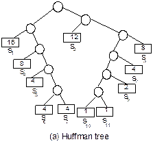

Fig. 8.54 Variable
length coding using Huffman tree.
Whenever a sender sends some message, first it encodes constituent symbols using Huffman coding. At the receiver end, the same Huffman tree is used in order to decode the receiving message.
Huffman codes have two important properties.
1. It is an optimal set of binary code with minimum average length. In case of the current example, average length of binary code is 4.
2. It has the prefix property, that is, no code appears as the prefix of other code. Or, in other words, suppose, C is the set of generated binary code, and for a given y Î C, there does not exist a x Î C such that x q z = y, for some non-empty binary string z. Here q represents the concatenation operation.
Advantages of Huffman coding
Potential advantages obtained from the Huffman coding are listed as below:
1. The Huffman coding has the minimum average length, so it involves minimum transmission time as well as less amount of storage space. For an example, suppose there is a message of 128 symbols; all the symbols are from S1, S2, ..., S11 (as listed in Tables 7.2 and 7.3). Using fixed length coding we need 128 ´ 4 = 512 bits for the massage. On the other hand, using variable length technique,
The number of bits required
= ![]()
=![]()
![]()
![]()
= 388 bits
So, approximately 60% less bits are required if variable length coding is used than the fixed length coding. This is why, some data compression technique adopts Huffman coding scheme.
It does not require any end-of-character delimiter although the binary codes are of variable length codes. This is because of its unique prefix property. In a simple linear scan of a Huffman encoded bit string, one can easily isolate the next coded data value. For example, on receiving the bit string ‘00111110 01010’ scanner easily identifies for first two bits ‘00’ as S1, next three bits ‘111’ for S3, next five bits ‘11001’ as S9 and the last three bits ‘010’ as S4. Scanning the codes for the next symbol starts from root and ends on reaching the external node.
Disadvantages of Huffman Coding
Of course, the main disadvantage with Huffman coding is that they are of variable length codes. Processing time is required for both encoding and decoding the message. Another difficulty that may arise with these codes is that, if a bit gets changed due to noise then it may not recognize the remaining part of the massage properly.